For large samples the maximum likelihood estimate is approximately normal, centred on the truth, with variance one over the information. Derive it from one Taylor step on the score, turn the curvature into standard errors, and carry them to other quantities with the delta method.
S02.10.3L2 Intermediate25 minIn review (what this means)
The maths and code on this page are checked by automated tests on every change, but an independent reader has not signed it off yet. Spot a mistake or a confusing step? Tell us.
State that for large n the MLE is approximately normal with mean theta and variance 1 / (n I(theta)), and the conditions this needs.
Derive the result informally from a first-order Taylor step on the score, the central limit theorem and the law of large numbers.
Compute a standard error from the observed information, 1 / sqrt(J), and for several parameters from the inverse of minus the Hessian.
Apply the delta method to find the standard error of a function of an estimate, and check it by simulation.
The question
Fit a logistic regression with a statistics package and every weight comes with a standard error beside it. Fit any model by maximum likelihood with an optimiser, and the same numbers can be read off its inverse Hessian. Where do they come from? The coin’s estimate 0.7 and the waiting times’ rate 0.5 deserve standard errors too: what are they, and when can we trust them?
From the last lesson
1. What does the Cramér-Rao bound say?
Show answer
An unbiased estimator from \(n\) independent observations has variance at least \({1/(n\,I(\theta))}\), under regularity conditions such as a support that does not depend on \(\theta\).
2. Is the unbiased estimator \({(n - 1)/\sum x_i}\) of an exponential rate efficient?
Show answer
No. Its variance is \({\lambda^2/(n - 2)}\) against the bound \({\lambda^2/n}\), an efficiency of \({(n - 2)/n}\), which approaches 1 only as \(n\) grows.
Intuition
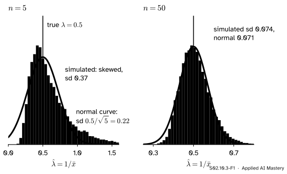
Draw many samples of waiting times from an exponential with true rate \({\lambda = 0.5}\), and compute the MLE \({\hat\lambda = 1/\bar x}\) of each. With 5 waiting times per sample, the estimates spread lopsidedly; with 50, they pile up into a bell.
S02.10.3-F1
The sampling distribution of the exponential rate’s MLE, simulated, under the normal curve with mean \(\lambda\) and variance \({1/(n I(\lambda)) = \lambda^2/n}\). At \({n = 5}\) the curve is a poor guide; at \({n = 50}\) it is a good one.
The normal curve in each panel was drawn without any simulation: its centre is the truth and its variance is the Cramér-Rao floor of lesson S02.10.2. As \(n\) grows the MLE’s sampling distribution becomes that curve. This is asymptotic normality, and it is why “estimate plus or minus 1.96 standard errors” works for almost every model fitted by maximum likelihood.
Build it up
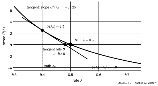
Step 1. The MLE solves an equation. At the estimate the score is zero: \({U(\hat\theta) = 0}\). For the waiting times, \({U(\lambda) = 5/\lambda - 10}\) is zero at \({\hat\lambda = 0.5}\).
Step 2. Near the truth the score is nearly a straight line. Call the true value \({\theta_0}\). A first-order Taylor step (M04.8) replaces the score by its tangent at \({\theta_0}\):
The Taylor step, drawn with \({\lambda_0 = 0.4}\) playing the truth. The tangent at the truth crosses zero at 0.48, close to where the score itself does, 0.5. The closer the two points, the better the straight line.
Step 3. Solve the straight line instead. Put \({\theta = \hat\theta}\), where the left side is 0:
Step 4. Read the top and the bottom. The top, \({U(\theta_0)}\), is a sum of \(n\) independent scores, each with mean 0 and variance \({I(\theta_0)}\) (lesson S02.10.1). The bottom, \({-U'(\theta_0) = -\ell''(\theta_0)}\), is a sum of \(n\) independent curvatures, each with mean \({I(\theta_0)}\). So the bottom is close to \({n I(\theta_0)}\), and the top is a centred sum with variance \({n I(\theta_0)}\). Dividing, the error \({\hat\theta - \theta_0}\) has mean about 0 and variance about \({n I / (nI)^2 = 1/(nI)}\).
The formal statement
NoteTheorem: asymptotic normality of the MLE
Let \({X_1, \dots, X_n}\) be independent draws from \({f(x \mid \theta_0)}\), under regularity conditions: the support does not depend on \(\theta\), \({\theta_0}\) is not on the edge of the parameter range, the log-likelihood is smooth, and \({I(\theta_0) > 0}\). Then as \({n \to \infty}\),
Top.\({U(\theta_0)/\sqrt n}\) is \({\sqrt n}\) times the mean of \(n\) independent scores with mean 0 and variance \({I(\theta_0)}\). By the central limit theorem (M06.11.3) it tends to \({N(0, I(\theta_0))}\).
Bottom.\({-\ell''(\theta_0)/n}\) is the mean of \(n\) independent curvatures with mean \({I(\theta_0)}\). By the law of large numbers it tends to the number \({I(\theta_0)}\).
Slutsky’s lemma (stated here; proofs of convergence are M07.5) says that if one sequence of random variables tends in distribution to \(Y\) and another tends to a constant \({c \neq 0}\), their ratio tends in distribution to \({Y/c}\). A normal variable with variance \({I}\) divided by the number \({I}\) has variance \({I/I^2 = 1/I}\), which is the theorem. Read with the Cramér-Rao bound, it says the MLE reaches the floor in the limit: it is asymptotically efficient.
Standard errors. The variance \({1/(nI(\theta_0))}\) involves the unknown truth. Replace it by what the data show: the observed information, the curvature at the peak,
Several parameters. With a vector \(\vect{\theta}\), the curvature is minus the Hessian matrix of \(\ell\) at the peak, and the approximate covariance matrix of \(\hat{\vect{\theta}}\) is its inverse, \({\mat{J}^{-1}}\). Each standard error is the square root of a diagonal entry of \({\mat{J}^{-1}}\). An optimiser that minimises the negative log-likelihood estimates this inverse Hessian, which is where its standard errors come from.
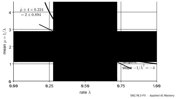
The delta method. To get the standard error of a function \({g(\hat\theta)}\), take the same Taylor step on \(g\): \({g(\hat\theta) \approx g(\theta_0) + g'(\theta_0)(\hat\theta - \theta_0)}\). A constant times an approximately normal error is approximately normal, so
The delta method for the mean waiting time \({\mu = 1/\lambda}\). Near \({\hat\lambda = 0.5}\) the curve is close to its tangent, of slope \(-4\), so one standard error of 0.224 in the rate becomes \({4 \times 0.224 = 0.894}\) in the mean.
Worked example
Standard errors for the coin, the waiting times, and the mean waiting time.
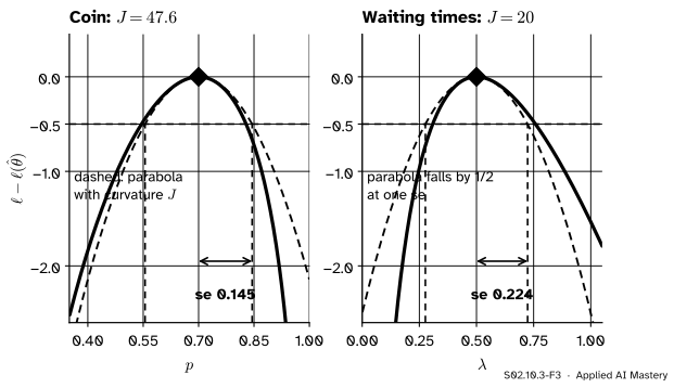
S02.10.3-F3
The parabola with the curve’s curvature \(J\) at the peak falls by exactly \({\tfrac12}\) one standard error \({1/\sqrt J}\) away. The true curves are lopsided; the parabolas are what the standard errors assume.
Coin.\(\ell''(p) = {-7/p^2} - {3/(1-p)^2}\), so at \({\hat p = 0.7}\), \(J = {7/0.49} + {3/0.09} = 14.29 + 33.33 = 47.6\), and \({\widehat{\mathrm{se}} = 1/\sqrt{47.6}}\)\(= 0.145\). This equals \({\sqrt{\hat p(1 - \hat p)/n}} = {\sqrt{0.021}}\), the familiar formula.
Waiting times.\({\ell(\lambda) = 5\ln\lambda - 10\lambda}\), so \({\ell''(\lambda) = -5/\lambda^2}\), and at \({\hat\lambda = 0.5}\), \({J = 5/0.25 = 20}\) and \({\widehat{\mathrm{se}} = 1/\sqrt{20} = 0.224}\).
Why the parabola falls by a half.\({-\tfrac12 J\,(\theta - \hat\theta)^2}\) at \({\theta - \hat\theta = 1/\sqrt J}\) is \({-\tfrac12 J / J = -\tfrac12}\).
Mean waiting time.\({\hat\mu = 1/\hat\lambda = 2}\) by invariance (S02.3.2). With \({g(\lambda) = 1/\lambda}\), \({g'(\lambda) = -1/\lambda^2 = -4}\) at 0.5, so \({\widehat{\mathrm{se}}(\hat\mu) = 4 \times 0.224 = 0.894}\). Check: \({\hat\mu = \bar x}\), and an exponential’s standard deviation equals its mean, so \({\widehat{\mathrm{se}}(\bar x) = 2/\sqrt 5 = 0.894}\) as well.
Code
From scratch: observed information from the formula and from a finite-difference second derivative.
J formula: 20.0   finite differences: 20.0   se: 0.224
coin: J = 47.62   se = 0.145
mean waiting time: se by the delta method = 0.894
Now the check by simulation: 20,000 samples with true rate 0.5 (seed 4), at \({n = 5}\) and \({n = 50}\).
for n in (5, 50): rng = np.random.default_rng(4) x = rng.exponential(2.0, size=(20_000, n)) lam_hats =1/ x.mean(axis=1)print(f"n = {n:2d}: mean {lam_hats.mean():.3f}, sd {lam_hats.std():.4f},"f" theory sd {0.5/ math.sqrt(n):.4f}; sd of 1/lambda-hat {x.mean(axis=1).std():.3f},"f" delta method {4*0.5/ math.sqrt(n):.3f}")if n ==5: sd5, mean5, mu_sd5 = lam_hats.std(), lam_hats.mean(), x.mean(axis=1).std()else: sd50 = lam_hats.std()
n =  5: mean 0.627, sd 0.3658, theory sd 0.2236; sd of 1/lambda-hat 0.895, delta method 0.894
n = 50: mean 0.510, sd 0.0736, theory sd 0.0707; sd of 1/lambda-hat 0.283, delta method 0.283
At \({n = 5}\) the estimates are biased upwards (mean about 0.63) and spread far more than the theory says (0.37 against 0.22). At \({n = 50}\) the theory is within 4%. The delta method for the mean waiting time is good already at \({n = 5}\), because \({1/\hat\lambda = \bar x}\) is a plain average.
Several parameters: the line through the four points of ML01.4 with normal noise of known \({\sigma = 1}\). Minus the Hessian of \(\ell\) in \({(w, b)}\) is \({\mat{X}\T\mat{X}}\), where \(\mat{X}\) has the inputs and a column of ones.
X = np.column_stack([[1, 2, 3, 4.0], np.ones(4)])H = X.T @ X # [[30, 10], [10, 4]]se_right = np.sqrt(np.diag(np.linalg.inv(H)))se_wrong =1/ np.sqrt(np.diag(H))print("H =", H.tolist(), " se from the inverse:", se_right.round(3), " 1/sqrt(diagonal):", se_wrong.round(3))
H = [[30.0, 10.0], [10.0, 4.0]] se from the inverse: [0.447 1.225] 1/sqrt(diagonal): [0.183 0.5 ]
Finally the optimiser’s version: scipy.optimize.minimize with BFGS keeps an estimate of the inverse Hessian of the function it minimises, here the negative log-likelihood of the waiting times.
BFGS builds its inverse Hessian from the steps it took, so it is an approximation; here it lands within a few thousandths of the exact 0.05, and the exact digits can differ between machines.
Explore
The interactive, curvature and intervals, is in lesson S02.10.4. Switch it to the waiting times and raise \(n\): the dashed parabola hugs the curve more and more closely, which is asymptotic normality seen in the likelihood itself.
Pitfalls
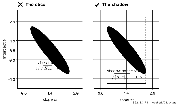
S02.10.3-F4
Wrong beside right. With correlated parameters the ellipse is tilted. Its slice at the best \(b\) is narrow, but \(b\) is not known; the honest uncertainty in \(w\) is the ellipse’s full shadow on the \(w\) axis, two and a half times wider.
“The standard error of a parameter is one over the square root of its diagonal Hessian entry.”
That is the uncertainty in \(w\)if \(b\) were known exactly. When parameters are correlated, as the slope and intercept of a line are, invert the whole matrix first and then take square roots of the diagonal: \({\sqrt{0.2} = 0.447}\), not \({1/\sqrt{30} = 0.183}\). The inverse’s diagonal entry is never smaller than one over the Hessian’s.
“The normal approximation holds for my sample.”
It is a large-sample result. With five waiting times the MLE of the rate is skewed, biased upwards, and spread 0.37 rather than 0.22. A useful check is the likelihood itself: if it is far from a parabola over the range of interest, as in the worked-example figure, the standard error is not to be trusted, and the likelihood-ratio interval of lesson S02.10.4 is safer.
“Every MLE is asymptotically normal.”
Only under the regularity conditions. For the uniform on \({[0, \theta]}\) the MLE is the sample maximum, its error shrinks like \({1/n}\) instead of \({1/\sqrt n}\), and its distribution is lopsided at every \(n\), because the support moves with \(\theta\). A true value on the edge of the parameter range breaks the theorem too. And when an estimate lands on the edge, such as \({\hat p = 0}\) after no heads, the score is not even zero at the peak, and the usual formula \({\sqrt{\hat p(1 - \hat p)/n}}\) gives a standard error of 0, which is plainly wrong.
Check yourself
Recall
1. What is the approximate distribution of the MLE for large \(n\)?
Show answer
Normal, centred on the true \(\theta\), with variance \({1/(n\,I(\theta))}\).
2. Which two limit theorems handle the top and the bottom of \({(\hat\theta - \theta_0) \approx U(\theta_0)/(-\ell''(\theta_0))}\)?
Show answer
The central limit theorem for the top, a sum of independent zero-mean scores; the law of large numbers for the bottom, a mean of curvatures that settles at \({I(\theta_0)}\). Slutsky’s lemma joins them.
3. How is a standard error computed from the data, and what is it for the coin?
Show answer
\({\widehat{\mathrm{se}} = 1/\sqrt{J(\hat\theta)}}\) with \({J = -\ell''(\hat\theta)}\); for 7 heads in 10, \({J = 47.6}\) and \({\widehat{\mathrm{se}} = 0.145}\).
4. With several parameters, where do the standard errors come from?
Show answer
From the square roots of the diagonal of the inverse of minus the Hessian of \(\ell\) at the peak.
5. State the delta method and use it for the mean waiting time.
Show answer
\({\widehat{\mathrm{se}}(g(\hat\theta)) \approx \abs{g'(\hat\theta)}\,\widehat{\mathrm{se}}(\hat\theta)}\). With \({g(\lambda) = 1/\lambda}\), \({\abs{g'(0.5)} = 4}\), so \({4 \times 0.224 = 0.894}\).
Exercises
1.★ A classifier gets 90 of 100 test examples right. Find the observed information and the standard error of the estimated accuracy.
Show solution
\(J = {90/0.9^2} + {10/0.1^2} = 111.1 + 1000 = 1111.1\), so \({\widehat{\mathrm{se}} = 1/\sqrt{1111.1}} = 0.030\), the same as \({\sqrt{0.9 \times 0.1/100}}\).
2.★★ The odds of heads are \({g(p) = p/(1 - p)}\). Estimate them from 7 heads in 10 tosses and give a standard error by the delta method.
Show solution
By invariance, the estimate is \({0.7/0.3 = 2.33}\). The derivative is \({g'(p) = 1/(1 - p)^2}\) (quotient rule), which is \({1/0.09 = 11.1}\) at 0.7. So \({\widehat{\mathrm{se}} \approx 11.1 \times 0.145 = 1.61}\). A standard error that large compared with 2.33 warns that the odds are poorly pinned down by 10 tosses, and that a normal approximation for them would be crude.
3.★★★ Design A’s five times, 4, 5, 7, 8 and 11 minutes, are modelled as normal with mean \(\mu\) and variance \({v = \sigma^2}\). The MLEs are \({\hat\mu = 7}\) and \({\hat v = 6}\) (S02.3.3). Using the information matrix of S02.10.1, find standard errors for both.
Show solution
For \(n\) observations the information matrix is \({n\,\mat{I}(\mu, v)}\), diagonal with entries \({n/v}\) and \({n/(2v^2)}\). Because it is diagonal its inverse is diagonal too, with entries \({v/n}\) and \({2v^2/n}\). At the estimates,
Sources. Each was opened and checked against this lesson on 15 November 2026.
Stanford STATS 200, Autumn 2016, Lecture 14: Consistency and asymptotic normality of the MLE. Theorem 14.1 states that \({\sqrt n(\hat\theta - \theta_0) \to N(0, 1/I(\theta_0))}\) under conditions including a common support and an interior \({\theta_0}\); Section 14.2 sketches the proof by a first-order Taylor expansion of \({0 = \ell'(\hat\theta)}\), the law of large numbers for the denominator, the central limit theorem for the numerator, and Slutsky’s lemma, stated in a footnote.
Stanford STATS 200, Autumn 2016, Lecture 15: Fisher information and the Cramer-Rao bound. Theorem 15.2 extends the result to several parameters with the inverse information matrix, and Section 15.1 shows that the upper-left entry of the inverse of a 2 by 2 information matrix is never smaller than one over the upper-left entry, the pitfall of the slice and the shadow.
Philippe Rigollet, Maximum likelihood estimation slides, MIT OpenCourseWare 18.650, Fall 2016. Slide 23 states the theorem with limiting covariance \({I(\theta^*)^{-1}}\) and lists its conditions: an identified model, a support that does not depend on \(\theta\), a true value not on the boundary, and an invertible information matrix.