A number computed from a random sample is itself random. Tell apart the population, one sample and the sampling distribution of a statistic, list one exactly for five flats, simulate one for a city of 500, and see why a test-set score has one too.
S02.1.1L2 Intermediate25 minIn review (what this means)
The maths and code on this page are checked by automated tests on every change, but an independent reader has not signed it off yet. Spot a mistake or a confusing step? Tell us.
Tell apart the population, one sample and the sampling distribution of a statistic, in a picture and in words.
List the exact sampling distribution of a sample mean for a small population by enumerating every possible sample.
Simulate the sampling distribution of a statistic with numpy.random.default_rng and its choice method.
Describe the two models of where data come from, a finite list and i.i.d. draws, and say why the second is the default.
Explain why a test-set score and a mini-batch gradient are statistics with sampling distributions.
The question
You draw 25 flats by lot from a city and find a mean rent of 9.23 (hundreds of euros a month). A colleague draws another 25 and gets 7.06. Neither of you made a mistake. So what is the number 9.23 a draw from, and how could you ever say how far it is from the city’s true mean rent?
Intuition
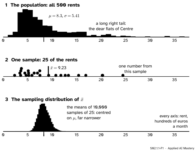
Three different distributions are in play whenever we learn from a sample, and almost every mistake in statistics comes from mixing them up. The picture shows all three on one scale.
S02.1.1-F1
Three distributions not to confuse. 1 The population: all 500 rents of the city. 2 One sample of 25, and the one number we compute from it, its mean \(\cmodel{\bar{x}}\). 3 The sampling distribution: where \(\bar{x}\) lands over 10,000 samples of 25.
The population (panel 1) is fixed. It has one mean, \(\ctruth{\mu} = 8.3\), and one spread, \(\ctruth{\sigma} = 5.41\). We usually cannot see it.
A sample (panel 2) is what we can see: 25 rents drawn by lot. From it we compute a number, here the mean \(\cmodel{\bar{x}} = 9.23\).
Now imagine drawing a fresh sample, and another, and another, each time computing \(\bar{x}\). Each sample holds different flats, so each \(\bar{x}\) is different. Collect them all and you get panel 3: the sampling distribution of \(\bar{x}\). It is centred on \(\mu\), and it is far narrower than the population, because a mean of 25 rents averages away most of the scatter of single rents.
Your 9.23 and your colleague’s 7.06 are two draws from panel 3. Everything that later lessons say about uncertainty is a statement about the shape and width of that panel.
Build it up
Step 1. A parameter belongs to the population. A parameter is a number that describes the population, such as \(\mu\), \(\sigma\) or the share \(p\) of flats above some rent. It does not change. (You met parameters and statistics in lesson S01.2.1.)
Step 2. A statistic belongs to the sample. A statistic is any number computed from the sample alone: the mean \(\bar{x}\), the median, the largest value, the share above 10.
Step 3. Before the draw, a statistic is random. Before the flats are chosen, we do not know which flats we will get, so we do not know \(\bar{x}\). As a rule applied to a random sample, \(\bar{X}\) is a random variable, just like the roll of a die. After the draw it takes one value, \(\bar{x}\). Capital letters name the random variable, small letters the value it took.
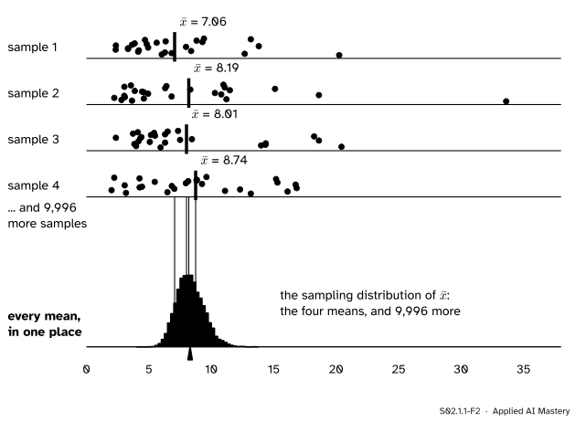
Step 4. A random variable has a distribution. The distribution of a statistic over all the samples the sampling scheme could produce is its sampling distribution. The picture below is the machine that makes one.
S02.1.1-F2
The sampling machine. Each sample of 25 gives one mean (vermillion tick). Drop every mean onto one axis and repeat 10,000 times: the pile is the sampling distribution of \(\bar{x}\).
Two things about the machine matter. The sample size \(\cparam{n}\) is fixed for every row: the sampling distribution of the mean of 25 rents is not that of the mean of 100. And every row follows the same rule for choosing flats, so the pile describes that rule.
The formal statement
NoteDefinitions
Let \(X_1, \dots, X_n\) be the values of a random sample. A statistic is a function \(T = t(X_1, \dots, X_n)\) of the sample that does not involve unknown parameters. Its sampling distribution is the probability distribution of \(T\) induced by the random choice of the sample. Once the sample is drawn, \(T\) takes the value \(t(x_1, \dots, x_n)\), an estimate when it is used to guess a parameter.
The sampling distribution depends on three things: the population, the statistic, and the rule that chooses the sample. Two rules recur.
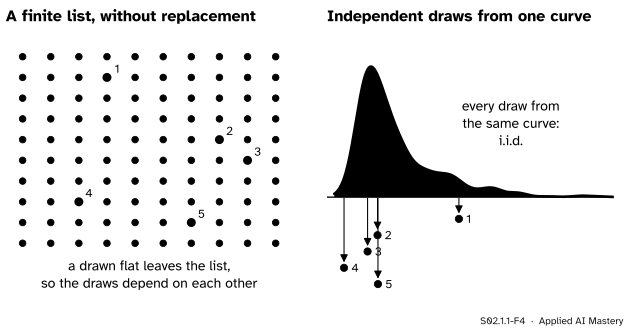
Model 1: a finite list, drawn without replacement. The population is a list of \(N\) units, and a simple random sample of size \(n\) is chosen so that every set of \(n\) units is equally likely. A unit that has been drawn cannot be drawn again, so the draws depend on each other: if the first flat is the penthouse, the second cannot be.
Model 2: independent draws from one distribution. The values \(X_1, \dots, X_n\) are independent and identically distributed (i.i.d.): each has the same distribution \(F\), and knowing some of them tells you nothing about the others. Drawing with replacement from a list is exactly this, with \(F\) the distribution of the values in the list: every draw sees the whole list again.
S02.1.1-F4
The two models of where data come from. Left: a list of units, each drawn at most once. Right: independent draws, each from the same distribution.
This course takes Model 2 as its default, for three reasons.
When the list is long, the two agree. For 25 flats from the city’s 500, lesson S02.1.2 shows that leaving out replacement changes the spread of \(\bar{x}\) by a factor of only 0.976.
Many data come from no list at all. The next toss of a coin, the next email a spam filter will see, tomorrow’s waiting time: these are draws from a process, and there is no finite list to exhaust.
The mathematics is simpler. Independence lets variances add (M06.7), which is what the rest of this module uses. Pishro-Nik’s textbook defines a random sample as i.i.d. draws, and notes that drawing with replacement is what makes the draws independent.
So from here on, unless a lesson says otherwise, “a sample of size \(n\)” means i.i.d. draws, and a simulation draws from the city with replacement.
Worked example
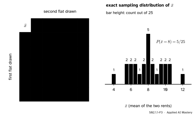
The exact sampling distribution for five flats. The five-flat population of S01 has rents 4, 7, 8, 9 and 12, with mean \(\ctruth{\mu} = 8\). Draw two flats with replacement and take their mean. List every sample, since there are only \(5 \times 5 = 25\) ordered draws, each with chance \(1/25\).
S02.1.1-F3
Every ordered draw of two from the five flats, with its mean (left), and the exact sampling distribution of \(\bar{x}\) that the table adds up to (right).
Fill the table. The cell in row \(a\) and column \(b\) holds \((a + b)/2\). For example, row 4 and column 9 give \((4 + 9)/2 = 6.5\).
Count each value. A value off the diagonal of the table appears twice, once in each order. The mean 8 appears five times: from \((4, 12)\) and \((12, 4)\), from \((7, 9)\) and \((9, 7)\), and from \((8, 8)\). So \(P(\bar{X} = 8) = 5/25 = 0.2\).
Read the distribution. The 13 possible means, each with its count out of 25, are 4 (1), 5.5 (2), 6 (2), 6.5 (2), 7 (1), 7.5 (2), 8 (5), 8.5 (2), 9 (1), 9.5 (2), 10 (2), 10.5 (2) and 12 (1). The counts add to 25.
Check the centre. The table is symmetric about 8: each mean \(8 + d\) is paired with a mean \(8 - d\) of the same count. So the 25 means average exactly 8, the population mean.
Ask a question of it. How likely is a sample mean within 1 of the truth? The values 7, 7.5, 8, 8.5 and 9 have counts \(1 + 2 + 5 + 2 + 1 = 11\), so the chance is \(11/25 = 0.44\). More than half the time, two flats miss the mean by more than 1.
Code
First the city, built exactly as in S01, so that every lesson uses the same 500 rents.
import itertoolsfrom collections import Counterfrom fractions import Fractionimport numpy as nprng = np.random.default_rng(0)rents = []for size, district_mean in ((250, 5), (150, 8), (100, 17)): # South, North, Centre draws = rng.gamma(9.0, 1.0, size) rents.append(draws * district_mean / draws.mean())rents = np.concatenate(rents)mu, sigma = rents.mean(), rents.std() # divisor N: the population's own spreadprint(f"N = {len(rents)}, mu = {mu:.2f}, sigma = {sigma:.2f}")
N = 500, mu = 8.30, sigma = 5.41
The five flats, by listing every ordered draw of two, with exact fractions.
five = [4, 7, 8, 9, 12]means = [Fraction(a + b, 2) for a, b in itertools.product(five, repeat=2)]counts = Counter(means)print(len(means), "draws;", len(counts), "different means")print("P(mean = 8) =", Fraction(counts[8], 25))print("average of the 25 means =", sum(means) /25)print("P(|mean - 8| <= 1) =", Fraction(sum(k for m, k in counts.items() ifabs(m -8) <=1), 25))
25 draws; 13 different means
P(mean = 8) = 1/5
average of the 25 means = 8
P(|mean - 8| <= 1) = 11/25
Now the city, where listing is hopeless: there are \(500^{25}\) ordered samples of 25. We simulate instead. rng.choice(rents, 25) draws 25 values with replacement, which is the method’s default (replace=True), and size=(10_000, 25) draws 10,000 such samples at once, one per row.
rng = np.random.default_rng(1)sample = rng.choice(rents, 25)print(f"your sample: mean {sample.mean():.2f}")colleague = np.random.default_rng(11).choice(rents, 25)print(f"your colleague's: mean {colleague.mean():.2f}")rng = np.random.default_rng(2)xbars = rng.choice(rents, size=(10_000, 25)).mean(axis=1)lo, hi = np.quantile(xbars, [0.025, 0.975])print(f"10,000 sample means: average {xbars.mean():.2f}, middle 95% from {lo:.2f} to {hi:.2f}")print(f"share within 2 of mu: {np.mean(np.abs(xbars - mu) <2):.2f}")
your sample: mean 9.23
your colleague's: mean 7.06
10,000 sample means: average 8.31, middle 95% from 6.41 to 10.62
share within 2 of mu: 0.94
The 10,000 means average 8.31, within simulation noise of \(\mu = 8.3\), and the middle 95 percent of them lie between 6.41 and 10.62. So a sample of 25 usually lands within about 2 of the truth: 94 percent of the simulated means did. The last digits of these simulated numbers depend on the seed; the pattern does not.
Explore
This module’s interactive, the sampling-distribution simulator, lives in lesson S02.1.3. It draws samples one at a time from 40 skewed rents, or tosses of a coin, and lets you watch the sampling distribution of the mean, the median, a proportion or the maximum grow sample by sample.
Pitfalls
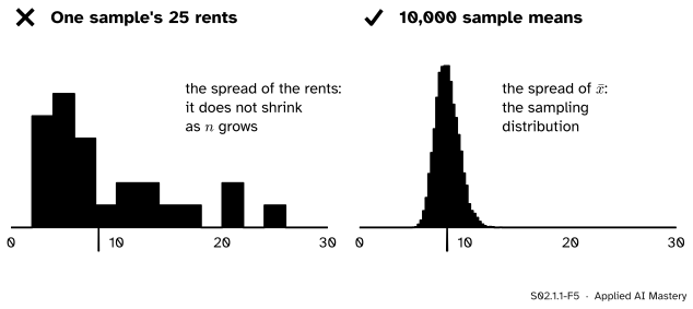
S02.1.1-F5
Wrong beside right. The histogram of one sample shows how rents vary. The sampling distribution shows how the mean varies from sample to sample, and it is far narrower.
“The sampling distribution is the histogram of my sample.”
The histogram of your sample estimates the population (panel 1), not the sampling distribution (panel 3). With more data it looks more like the population, and its spread settles near \(\sigma = 5.41\); it never narrows. The sampling distribution of \(\bar{x}\) narrows as \(n\) grows. You never see it directly from one sample. You reason about it, as the next lesson does, or simulate it, as the bootstrap of S02.8 does.
“A statistic is just a number.”
The value you computed, 9.23, is a number. The statistic, “the mean of 25 flats drawn by lot”, is a random variable whose value depends on which flats came up. Every claim of the form “how sure are we?” is about the random variable, not the one number.
“My model’s test accuracy is its accuracy.”
A test-set score is a statistic: the share of correct answers on the examples that happened to land in the test set. Another random split gives another score, so the score has a sampling distribution around the accuracy the model would have on all future data. That is why two runs of the same pipeline can disagree by a point or two, and why the gap between training and test scores (ML01.2.3) is itself noisy. The same holds for a mini-batch gradient (ML01.5.4): it is the mean of the gradients of \(\abs{B}\) examples drawn at random, so it scatters around the full gradient with a sampling distribution of its own.
Check yourself
Recall
1. Name the three distributions of the anchor picture and say which one is fixed.
Show answer
The population (fixed), one sample, and the sampling distribution of the statistic over many samples.
2. What makes a number a statistic rather than a parameter?
Show answer
A statistic is computed from the sample alone; a parameter describes the population.
3. For two flats drawn with replacement from 4, 7, 8, 9, 12, what is \(P(\bar{X} = 8)\), and why?
Show answer
\(5/25 = 0.2\): the ordered draws \((4, 12)\), \((12, 4)\), \((7, 9)\), \((9, 7)\) and \((8, 8)\) give 8.
4. What does i.i.d. mean, and which way of drawing from a list gives i.i.d. values?
Show answer
Independent and identically distributed: every value has the same distribution and none tells you anything about another. Drawing with replacement gives i.i.d. values.
5. Why does a test-set accuracy have a sampling distribution?
Show answer
It is computed from the examples that happened to land in the test set; a different random test set would give a different value.
Exercises
1.★ For two flats drawn with replacement from 4, 7, 8, 9, 12, find \(P(\bar{X} \ge 10)\).
Show solution
The means of at least 10 are 10, 10.5 and 12, with counts 2, 2 and 1 out of 25 (from \((8, 12)\) and \((12, 8)\), \((9, 12)\) and \((12, 9)\), and \((12, 12)\)). So \(P(\bar{X} \ge 10) = 5/25 = 0.2\).
2.★★ Now draw the two flats without replacement, so that each of the ten unordered pairs is equally likely. List the sampling distribution of \(\bar{X}\) and find \(P(\abs{\bar{X} - 8} \le 1)\). Compare with 0.44 for the draws with replacement.
Show solution
The ten pairs give means 5.5, 6, 6.5, 8 (from 4 and 12), 7.5, 8 (from 7 and 9), 9.5, 8.5, 10 and 10.5. So 8 has chance \(2/10\) and each other value \(1/10\). The means within 1 of 8 are 7.5, 8, 8 and 8.5, so the chance is \(4/10 = 0.4\). It is lower than 0.44 because without replacement the “same flat twice” samples, which include \((8, 8)\) and the means 7 and 9, are impossible.
3.★★★ Write a function sampling_distribution(values, n) that returns, as a dictionary of exact fractions, the sampling distribution of the mean of \(n\) draws with replacement from values, by listing every ordered sample. Use it to show that for the five flats with \(n = 3\) the means still average exactly 8.
Show solution
import itertoolsfrom collections import Counterfrom fractions import Fractiondef sampling_distribution(values, n): total =len(values) ** n counts = Counter(Fraction(sum(s), n) for s in itertools.product(values, repeat=n))return {m: Fraction(k, total) for m, k insorted(counts.items())}dist = sampling_distribution([4, 7, 8, 9, 12], 3)print(sum(m * p for m, p in dist.items())) # 8
There are \(5^3 = 125\) ordered samples. The average is exactly 8 because each position of the sample is equally likely to hold each flat, so each of the three draws has mean 8, and the mean of their average is 8 by linearity of expectation (M06.7).
Summary card
A statistic is a random variable; its distribution over samples is its sampling distribution.
S02.1.1-F1
Population, sample, sampling distribution.
Parameter: a number of the population (\(\mu\), \(\sigma\), \(p\)). Statistic: a number of the sample (\(\bar{x}\), the median, \(\hat{p}\)).
Sampling distribution: where the statistic lands over all samples of size \(n\).
Five flats, two draws: 25 equally likely means, \(P(\bar{X} = 8) = 0.2\), centred on 8.
Default model: i.i.d. draws, the same as drawing with replacement from a list.
Sources and next steps
Sources. Each was opened and checked against this lesson on 15 November 2026.
David Diez, Mine Cetinkaya-Rundel and Christopher Barr, OpenIntro Statistics, 4th edition, Section 5.1.2: a simulation repeated 10,000 times, and the distribution of the resulting sample proportions called a sampling distribution, described by its centre, spread and shape.
Hossein Pishro-Nik, Introduction to Probability, Statistics, and Random Processes, Section 8.1.1: a random sample defined as i.i.d. random variables; sampling with replacement makes the draws independent, and for a large population sampling without replacement gives nearly the same results.
Next.S02.1.2 The standard error measures the width of the sampling distribution, derives it with and without replacement, and turns it into the square-root law.