A p-value mixes the size of an effect with the size of the sample. Report the effect in its own right: the raw difference with its interval, the standardised effect, the difference, relative risk and odds ratio for proportions, and the AUC as an effect size for ranks.
S02.6.2L2 Intermediate25 minIn review (what this means)
The maths and code on this page are checked by automated tests on every change, but an independent reader has not signed it off yet. Spot a mistake or a confusing step? Tell us.
Compute the raw difference of means, its interval and the standardised effect (Cohen’s d) for two groups.
Show that the two-sample t statistic is the standardised effect times the square root of n/2, so a p-value mixes effect and sample size.
State the conventional small, medium and large effects and say why they are only a last resort.
Describe a difference of two proportions as a difference, a relative risk and an odds ratio, and say what each hides.
Read the AUC as the probability that a draw from one group beats a draw from the other.
The question
Two experiments on web pages. In the first, the two page designs of S02.4.4 were shown to five visitors each: design B kept people three minutes longer, with p-value 0.12, “not significant”. In the second, a site showed two versions to 10,000 visitors each and got p-value 0.0004, “highly significant”. Which change made the bigger difference to the people using it? The p-values point one way. The effects point the other.
From the last lesson
1. What is the power of a test against an alternative?
Show answer
The probability that the test rejects \(H_0\) when that alternative is true, \(1 - \beta\).
2. For two groups of \(n\), how far apart are the null and alternative curves, in standard errors?
Show answer
\(\lambda = \delta\sqrt{n/2}\), where \(\delta = \Delta/\sigma\) is the standardised effect.
Intuition
An effect size says how big a difference is, in a way that does not grow with the sample. Picture the two populations the samples came from.
S02.6.2-F1
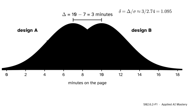
The two page designs. The gap between the centres is 3 minutes. Each group’s spread is about 2.74 minutes, so the gap is 1.095 standard deviations: the bells overlap, but not by much.
Two numbers describe the picture. The raw effect\(\Delta\) is the gap between the centres, 3 minutes. The standardised effect\(\delta = \Delta/\sigma\) is the same gap measured with the spread as the ruler: 1.095 standard deviations. Neither number knows how many visitors were watched. Adding visitors would make the dots more numerous and the estimates sharper, but the bells would stay where they are.
The p-value is different. It asks how surprising the data would be if there were no gap, and a gap of the same size becomes more surprising the more data show it.
Build it up
Step 1. The raw difference, with its interval. Design B’s mean is 10 minutes and A’s is 7, so \(\hat{\Delta} = 3\). Lesson S02.4.4 gave its 95 percent interval: \(-0.99\) to \(6.99\) minutes. That interval is the honest summary: the data fit anything from a one-minute loss to a seven-minute gain.
Step 2. Divide by the spread. Both sample variances are 7.5, so the pooled standard deviation is \(\sqrt{7.5} = 2.739\) and the estimated standardised effect, Cohen’s d, is \({3/2.739} = 1.095\). Minutes have gone; the effect now compares with any other study, on any scale.
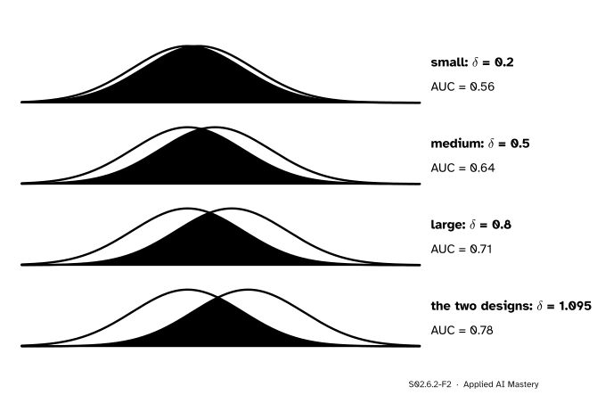
Step 3. Name it, with care. Cohen offered labels for when nothing else is known: 0.2 small, 0.5 medium, 0.8 large.
S02.6.2-F2
Cohen’s benchmarks as bells. Even a “large” effect leaves most of the two groups overlapping. The green number is the chance that a random member of the second group beats a random member of the first.
The labels are a last resort. A “small” effect of 0.1 on a death rate is enormous; a “large” one on a lab measure no one cares about is not. Compare an effect with others in the same field, and say what it means in the units people use.
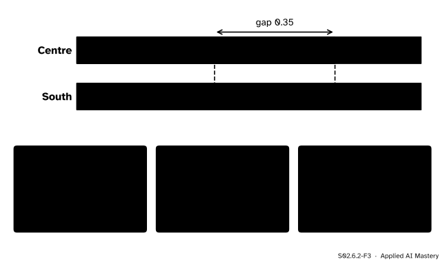
Step 4. Proportions have three effect sizes. For a yes-or-no outcome there is no standard deviation to divide by. The balcony table of S01.5.4 (invented) has 18 of 24 Centre flats with a balcony and 24 of 60 in South.
S02.6.2-F3
One comparison, three numbers. The difference is in percentage points, the relative risk is a ratio of shares, and the odds ratio is a ratio of odds.
The formal statement
NoteDefinitions: effect sizes for two groups
For means \(\mu_A, \mu_B\) and a common standard deviation \(\sigma\), the raw effect is \(\Delta = \mu_B - \mu_A\) and the standardised effect is \(\delta = \Delta/\sigma\). From samples of sizes \(n_A, n_B\), Cohen’s d estimates \(\delta\) by
For proportions \(p_A, p_B\): the difference \({p_B - p_A}\), the relative risk \({p_B/p_A}\) and the odds ratio, the ratio of the odds \({p/(1-p)}\) of the two groups.
Why a p-value mixes effect and size. With \(n\) in each group, the pooled two-sample t statistic (S02.7.1) divides the difference by its standard error \({s_p\sqrt{2/n}}\). Pull the standardised effect out:
The p-value is \({2\,\Prob(T_{2n-2} \ge \abs{t})}\), so it depends on \(\hat{\delta}\) only through the product \(\hat{\delta}\sqrt{n/2}\), and on \(n\) through that product and the degrees of freedom. A fixed effect gives an ever smaller p-value as \(n\) grows, and a tiny effect reaches any p-value you like with enough data.
S02.6.2-F5
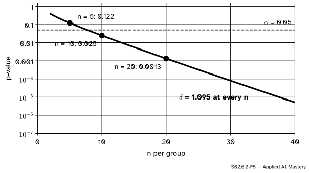
The two designs’ effect, \(\hat\delta = 1.095\), held fixed while the number of visitors per group grows. The effect never changes; the p-value falls through 0.05 between 5 and 10 visitors.
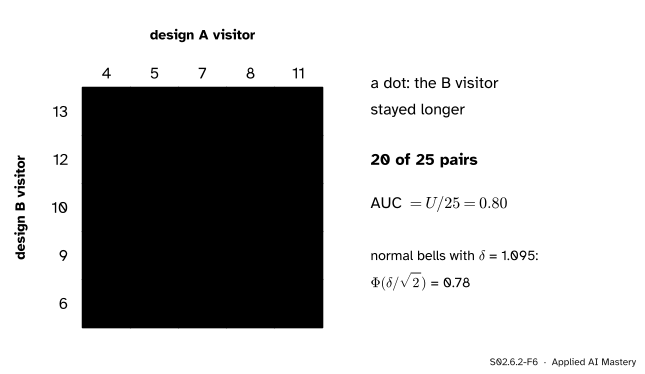
The AUC as an effect size for ranks. Another way to say how far apart two groups are: pick one member of each at random and ask how often the B member is larger. For the ten times this is a count over the \({5 \times 5} = 25\) pairs.
S02.6.2-F6
Every pairing of a B visitor with an A visitor. B wins 20 of the 25 pairs, so the estimated probability that a B visitor stays longer is 0.8.
That share is the Mann-Whitney \(U\) divided by \({n_A n_B}\) (S02.7.4), and it is the AUC of a classifier that scores visitors by their time (ML01.7). It needs no normality and no standard deviation. For two normal populations with a common \(\sigma\) it is tied to \(\delta\): the difference \({X_B - X_A}\) of independent draws is normal with mean \(\Delta\) and variance \({2\sigma^2}\). So \({Z = (X_B - X_A - \Delta)/(\sigma\sqrt{2})}\) is standard normal, and
For \(\delta = 1.095\) that is 0.78, close to the 0.80 counted from the data.
Worked example
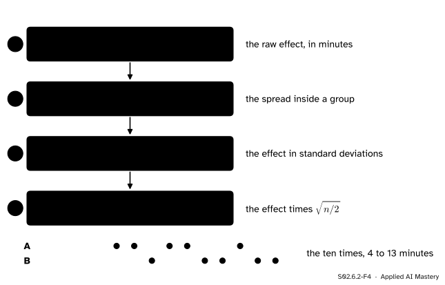
The two designs, then the same effect at other sizes.
S02.6.2-F4
From ten times to an effect size and a test statistic. Steps 1 to 3 do not depend on how many visitors there were; step 4 does.
Means 7 and 10, so \(\hat{\Delta} = 3\) minutes.
Both variances are 7.5, so \({s_p^2 = (4 \times 7.5 + 4 \times 7.5)/8} = 7.5\) and \(s_p = 2.739\).
\(\hat{\delta} = {3/2.739} = 1.095\): a large effect by Cohen’s labels.
\(t = {1.095 \times \sqrt{5/2}} = 1.732\) on 8 degrees of freedom, p-value 0.122.
Now keep \(\hat{\delta} = 1.095\) and imagine 10 visitors per group: \(t = {1.095 \times \sqrt{5}} = 2.449\) on 18 degrees of freedom, p-value 0.025. With 20 per group, \(t = 3.464\) and the p-value is 0.0013. Same effect, three verdicts.
The site test of the question had \(\hat{\delta} = 0.05\) with 10,000 per group: \(t = {0.05 \times \sqrt{5000}} = 3.54\) and p-value 0.0004. The p-value is 300 times smaller than the designs’, and the effect is 22 times smaller. Its AUC is \({\Phi(0.05/\sqrt{2})} = 0.51\): a visitor of the new version outstays one of the old version barely more often than a coin toss would say.
Code
From scratch with NumPy: the effect sizes, the t statistic as \(\hat{\delta}\sqrt{n/2}\), and the AUC as a count over pairs. The t distribution’s tail comes from SciPy.
import mathimport numpy as npfrom scipy import statsA = np.array([4, 5, 7, 8, 11])B = np.array([6, 9, 10, 12, 13])n =len(A)raw = B.mean() - A.mean()s_p = math.sqrt(((n -1) * A.var(ddof=1) + (n -1) * B.var(ddof=1)) / (2* n -2))d_hat = raw / s_pt = d_hat * math.sqrt(n /2)p_value =2* stats.t.sf(t, 2* n -2)auc = np.mean(B[:, None] > A[None, :]) # every pair (b, a): does b beat a?print(f"raw {raw}, s_p {s_p:.3f}, d {d_hat:.3f}, t {t:.3f}, p-value {p_value:.3f}, AUC {auc}")for size in (5, 10, 20): t_n = d_hat * math.sqrt(size /2)print(f"{size:2d} per group: t {t_n:.3f}, p-value {2* stats.t.sf(t_n, 2* size -2):.4f}")
raw 3.0, s_p 2.739, d 1.095, t 1.732, p-value 0.122, AUC 0.8
 5 per group: t 1.732, p-value 0.1215
10 per group: t 2.449, p-value 0.0248
20 per group: t 3.464, p-value 0.0013
The library agrees: scipy.stats.ttest_ind pools the variances by default and returns the same t.
1.732 0.122
site test: t 3.54  p-value 0.0004  AUC 0.51
For proportions, the three measures from the balcony table, and an error rate falling from 0.10 to 0.09:
def three_measures(p_a, p_b): odds =lambda p: p / (1- p)return p_b - p_a, p_b / p_a, odds(p_b) / odds(p_a)print("Centre against South:", [round(v, 3) for v in three_measures(24/60, 18/24)])print("errors 0.10 to 0.09: ", [round(v, 3) for v in three_measures(0.10, 0.09)])
Centre against South: [0.35, 1.875, 4.5]
errors 0.10 to 0.09:  [-0.01, 0.9, 0.89]
Explore
The module’s interactive, the power explorer, is in lesson S02.6.1. Set \(\delta\) to Cohen’s 0.2, 0.5 and 0.8 in turn and read the sample size for 80 percent power: about 393, 63 and 25 per group. The effect size, not the p-value, is what a study must be planned for.
Pitfalls
S02.6.2-F7
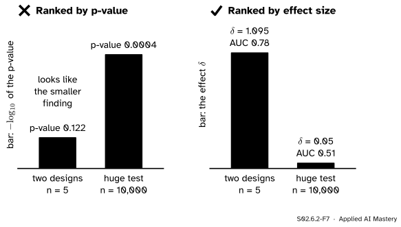
Wrong beside right. Ranked by p-value, the huge test looks like the stronger finding. Ranked by effect size, the designs’ change is 22 times larger.
“The smaller p-value means the bigger effect.”
A p-value measures surprise under \(H_0\), which grows with \(\hat{\delta}\sqrt{n/2}\). Report the effect and its interval beside the p-value; S02.5.4 made the same point for intervals.
“Our model makes 10 percent fewer errors.”
An error rate falling from 0.10 to 0.09 is a relative risk of 0.9, so “10 percent fewer”, but the difference is one percentage point. Relative measures hide the base rate. Report the difference with the two rates, as ML papers should when they quote an improvement.
“δ is 0.8, so the effect is large and important.”
Cohen’s labels are arbitrary conventions for when nothing better is known. Whether 0.8 matters depends on what is measured and what else in the field achieves; say it in the outcome’s own units.
“Cohen’s d from five visitors per group pins the effect down.”
It is an estimate with the uncertainty of its sample. Dividing the interval for \(\Delta\) by \(s_p = 2.74\) gives roughly \(-0.36\) to \(2.55\): from a small loss to an enormous gain.
Check yourself
Recall
1. What is the difference between the raw effect and the standardised effect?
Show answer
The raw effect \(\Delta\) is the difference of means in the outcome’s units; the standardised effect \(\delta = \Delta/\sigma\) divides it by the spread, so it has no units.
2. How are the two-sample t statistic and Cohen’s d related for \(n\) per group?
Show answer
\(t = \hat{\delta}\sqrt{n/2}\).
3. What are Cohen’s conventional small, medium and large effects?
Show answer
0.2, 0.5 and 0.8 standard deviations.
4. Name three effect sizes for a difference of two proportions.
Show answer
The difference, the relative risk (ratio of the proportions) and the odds ratio (ratio of the odds).
5. What does an AUC of 0.8 between two groups mean?
Show answer
A random member of the second group beats a random member of the first 80 percent of the time.
Exercises
1.★ Two groups of 20 have means 52 and 49 and a pooled standard deviation of 6. Find \(\hat{\delta}\), \(t\) and the two-sided p-value, and compare with the two designs.
Show solution
\(\hat{\delta} = {3/6} = 0.5\), medium. \(t = {0.5 \times \sqrt{20/2}} = 1.581\) on 38 degrees of freedom, p-value 0.12. The designs had p-value 0.12 too, with an effect more than twice as large: equal p-values, different effects, because the samples differ in size.
2.★★ Model A errs on 50 of 1,000 test examples and model B on 40 of 1,000. Give the difference, the relative risk and the odds ratio of B’s errors to A’s, and write one honest sentence about the improvement.
Show solution
The error rates are 0.05 and 0.04. Difference \({0.04 - 0.05} = -0.01\), relative risk \({0.04/0.05} = 0.8\), odds ratio \({(0.04/0.96)/(0.05/0.95)} = 0.792\). Honest: “B’s error rate is 4.0 percent against A’s 5.0 percent, one percentage point lower (a fifth fewer errors).”
3.★★★ Two normal populations share \(\sigma\). Show that the probability that a draw from B beats a draw from A is \(\Phi(\delta/\sqrt{2})\), and find the \(\delta\) that gives an AUC of 0.9.
Show solution
\(X_B - X_A\) is a difference of independent normals, so it is normal with mean \({\mu_B - \mu_A} = \Delta\) and variance \({\sigma^2 + \sigma^2} = 2\sigma^2\). Standardise: \({\Prob(X_B - X_A > 0)} = {\Prob(Z > -\Delta/(\sigma\sqrt{2}))}\), which is \({1 - \Phi(-\delta/\sqrt{2})} = \Phi(\delta/\sqrt{2})\) by the symmetry of \(\Phi\). For an AUC of 0.9, \({\delta/\sqrt{2}} = z_{0.9} = 1.2816\), so \(\delta = 1.81\): almost two standard deviations.
Summary card
An effect size says how big; a p-value says how surprising.
S02.6.2-F1
The gap, measured in spreads.
Standardised effect.\(\hat{\delta} = {(\bar{x}_B - \bar{x}_A)/s_p}\); 0.2, 0.5, 0.8 as a last resort.
Test statistic.\(t = \hat{\delta}\sqrt{n/2}\): effect times size.
Ranks. AUC \(= {U/(n_A n_B)}\); for normals \(\Phi(\delta/\sqrt{2})\).
Sources and next steps
Sources. Each was opened and checked against this lesson on 15 November 2026.
Daniël Lakens, Calculating and reporting effect sizes to facilitate cumulative science: a practical primer for t-tests and ANOVAs, Frontiers in Psychology 4:863 (open access). The section on Cohen’s d in between-subjects designs divides the difference of means by the pooled standard deviation; the section on interpreting Cohen’s d gives the benchmarks 0.2, 0.5 and 0.8, warns that they are arbitrary, and recommends the common language effect size, the probability that a member of one group scores higher than a member of the other.
SciPy, scipy.stats.ttest_ind. With the default equal_var=True it performs the standard independent two-sample test that assumes equal population variances, the pooled test used in the code.
Next.S02.6.3 Choosing the sample size turns the power formula round: given the effect worth finding, how many observations are needed?