\( \newcommand{\vect}[1]{\boldsymbol{\mathbf{#1}}} \newcommand{\mat}[1]{\boldsymbol{\mathbf{#1}}} \newcommand{\R}{\mathbb{R}} \newcommand{\E}{\mathbb{E}} \newcommand{\Prob}{\mathbb{P}} \newcommand{\T}{^{\top}} \newcommand{\norm}[1]{\lVert #1 \rVert} \newcommand{\abs}[1]{\lvert #1 \rvert} \newcommand{\ihat}{\mkern1mu\hat{\boldsymbol{\imath}}\mkern2mu} \newcommand{\jhat}{\mkern1mu\hat{\boldsymbol{\jmath}}\mkern2mu} \newcommand{\pd}[2]{\frac{\partial #1}{\partial #2}} \newcommand{\argmax}{\operatorname*{arg\,max}} \newcommand{\argmin}{\operatorname*{arg\,min}} \newcommand{\cdata}[1]{\class{c-data}{#1}} \newcommand{\cmodel}[1]{\class{c-model}{#1}} \newcommand{\ctruth}[1]{\class{c-truth}{#1}} \newcommand{\cgrad}[1]{\class{c-grad}{#1}} \newcommand{\closs}[1]{\class{c-loss}{#1}} \newcommand{\cparam}[1]{\class{c-param}{#1}} \newcommand{\csecond}[1]{\class{c-second}{#1}} \renewcommand{\,}{\mkern3mu} \)

The likelihood function

Fix the data and let the parameter vary: the probability of what you saw becomes the likelihood, a curve over the parameter. Draw it for a coin with 7 heads in 10 tosses, see why logarithms keep its peak, derive the estimate k / n, and compare two values by a ratio.

S02.3.1L2 Intermediate25 min

In review

The maths and code on this page are checked by automated tests on every change, but an independent reader has not signed it off yet. Spot a mistake or a confusing step? Tell us.

Before this lesson: S02.2 Point estimation: bias, variance and mean squared error M04.4 Optimization in one dimension M06.8 Common distributions and their stories

What you will be able to do

Define the likelihood as the probability (or density) of the observed data, read as a function of the parameter, and explain why it is not a probability distribution over the parameter.
Write the likelihood and log-likelihood of k heads in n tosses and explain why taking logarithms does not move the peak.
Derive the maximum likelihood estimate k / n for any k and n, and confirm the maximum with the second derivative.
Compare two parameter values by their likelihood ratio, and find the peak on a grid with numpy.argmax.

The question

A coin is tossed 10 times and lands heads 7 times. Every chance of heads \(p\) between 0 and 1 could have produced that, so which one should we believe? The answer, “the \(p\) that makes what we saw most probable”, is the most used idea in statistics. It is also how almost every machine-learning model is trained. What exactly is being made “most probable”, and why is the answer 0.7?

Intuition

Write the probability of the data as a formula with two kinds of input: the data and the parameter. Before the tosses we fix the parameter and ask about the data. After them the data are fixed, and the same formula, read the other way, scores every value of the parameter.

S02.3.1-F1

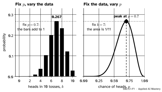
One formula, \({\binom{10}{k}\, p^k (1-p)^{10-k}}\), read two ways. Left: fix \(p\) and vary the count \(k\), and you get a probability distribution over the data. Right: fix the data at \({k = 7}\) and vary \(p\), and you get the likelihood. The dark bar and the peak are the same number.

The left panel is a probability distribution: it says how likely each count of heads would be if \(p\) were 0.7, and its bars add to 1. The right panel is the likelihood: the probability of the one count we did see, as \(p\) slides from 0 to 1. Its height at a value of \(p\) measures how well that value explains the data. It is tiny near \({p = 0.2}\), where 7 heads would be a fluke, and largest at \({p = 0.7}\).

That is the whole idea of maximum likelihood: estimate the parameter by the value at the top of the likelihood curve. The right panel is not a distribution over \(p\), though. Its area is 1/11, not 1, and nothing in it says how probable any value of \(p\) is.

Build it up

Step 1. One sequence. Say the tosses came out H H T H H H T H H T. They are independent, so their probability is a product of ten factors, \(p\) for each head and \({1 - p}\) for each tail:

\[ p^7 (1 - p)^3 . \]

Step 2. The likelihood. Read as a function of \(p\) with the tosses held fixed, that product is the likelihood, written \(\mathcal{L}(p)\). A curly L keeps it apart from a loss, which this course writes \(L\). If only the count of heads was recorded, every value gains the factor \({\binom{10}{7} = 120}\), the number of orders the 7 heads could come in. A constant factor stretches the curve but cannot move its peak, so the two versions give the same estimate.

Step 3. Logarithms. A product is awkward to differentiate and, for many data points, too small for a computer to hold. The logarithm turns the product into a sum,

\[ \ell(p) = \ln \mathcal{L}(p) = 7 \ln p + 3 \ln(1 - p), \]

the log-likelihood. Since \(\ln\) is increasing, a larger likelihood always has a larger logarithm, so the two curves peak at the same \(p\). Each toss now adds one term: each head adds \(\ln p\) and each tail adds \({\ln(1 - p)}\).

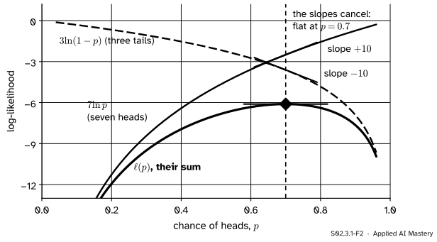
Step 4. A tug of war. The heads pull \(\ell\) up as \(p\) grows and the tails pull it down. The peak is where the two pulls balance.

S02.3.1-F2

The log-likelihood is a sum of the heads’ part and the tails’ part. At \({p = 0.7}\) the heads’ part climbs with slope \({7 / 0.7 = 10}\) and the tails’ part falls with slope \({3 / 0.3 = 10}\), so their sum is flat: that is the peak.

The formal statement

Definition: likelihood and maximum likelihood estimate

Let data \(x\) come from a model with probability (or density) \(f(x \mid \theta)\) for a parameter \(\theta\). With the data held fixed, the likelihood is the function

\[ \mathcal{L}(\theta) = f(x \mid \theta), \]

and the log-likelihood is \({\ell(\theta) = \ln \mathcal{L}(\theta)}\). For independent observations \({x_1, \dots, x_n}\) the likelihood is the product of their probabilities, so the log-likelihood is the sum of their logarithms. The maximum likelihood estimate (MLE) \(\hat{\theta}\) is the value of \(\theta\) with the largest likelihood.

Result: the MLE of a coin is the share of heads. Take \(k\) heads in \(n\) tosses with \({0 < k < n}\). Then

\[ \ell(p) = k \ln p + (n - k) \ln(1 - p) \]

on \({0 < p < 1}\). Differentiate term by term, using \({\tfrac{d}{dp}\ln(1 - p) = -\tfrac{1}{1 - p}}\) (the chain rule):

\[ \ell'(p) = \frac{k}{p} - \frac{n - k}{1 - p}. \]

Set it to zero and clear the fractions by multiplying both sides by \({p(1 - p)}\):

\[ \begin{aligned} k(1 - p) - (n - k)\,p &= 0 \\ k - kp - np + kp &= 0 \\ k &= np . \end{aligned} \]

So the only flat point is \({\cmodel{\hat{p}} = \cdata{k} / n}\). The second derivative is

\[ \ell''(p) = -\frac{k}{p^2} - \frac{n - k}{(1 - p)^2}, \]

a sum of two negative terms, so it is negative for every \(p\). The curve bends down everywhere, and the flat point is its one maximum. For the coin, \({\hat{p} = 7/10 = 0.7}\) and \({\ell''(0.7) = -7/0.49 - 3/0.09 \approx -47.6}\). How sharply the curve bends at its peak turns out to measure how precise the estimate is; lesson S02.10 makes that exact.

S02.3.1-F5

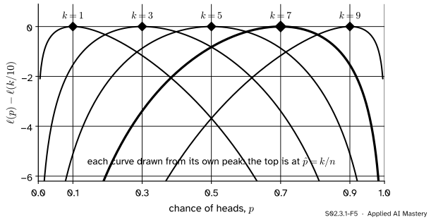
The log-likelihood for every count of heads in 10 tosses, each drawn from its own peak. The peak is always at the share of heads, \({\hat{p} = k/n}\).

Comparing two values: the likelihood ratio. The height of \(\mathcal{L}\) means nothing on its own: it changes if we record the sequence instead of the count. A ratio of two heights does not, because the constant cancels. The ratio

\[ \frac{\mathcal{L}(0.7)}{\mathcal{L}(0.5)} = \frac{0.7^7 \times 0.3^3}{0.5^{10}} = 2.28 \]

says that the observed tosses are 2.28 times as probable if \({p = 0.7}\) as if the coin is fair. That is a statement about the data under two hypotheses, not about which hypothesis is true. In logs the ratio becomes a difference, \({\ell(0.7) - \ell(0.5) = 0.823}\), and \({e^{0.823} = 2.28}\).

Go deeper: why the area under the likelihood is 1/11

The area under \({\binom{n}{k} p^k (1 - p)^{n - k}}\) from 0 to 1 is \({1/(n + 1)}\) for every \(k\). Here is a short argument. Draw \({n + 1}\) numbers uniformly from 0 to 1: one called \(P\) and \(n\) others. Given \({P = p}\), the chance that exactly \(k\) of the others fall below it is the binomial probability, so averaging over \(p\), the area is the chance that exactly \(k\) of the others are below \(P\). That is the chance that \(P\) is the \({(k + 1)}\)-th smallest of the \({n + 1}\) numbers, and by symmetry each of the \({n + 1}\) places is equally likely: \({1/(n + 1)}\). For 10 tosses that is 1/11. The area depends on \(n\) and on the constant in front, which is one more sign that the likelihood is not a density for \(p\).

Worked example

Find the MLE for 7 heads in 10 tosses, first by trying values, then by calculus.

S02.3.1-F3

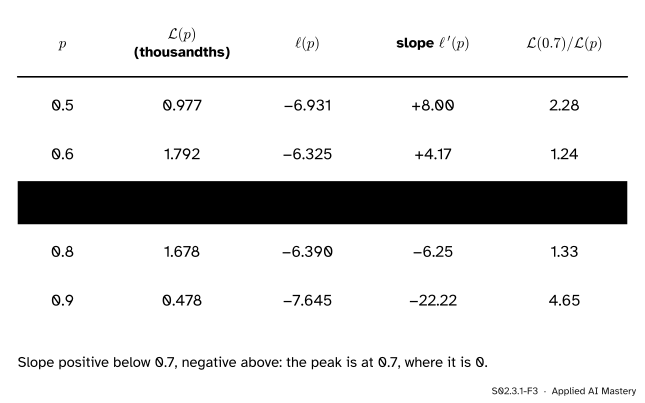
The coin’s likelihood, log-likelihood and slope at five values of \(p\). The slope changes sign at 0.7, and every other value explains the data less well.

Try values. At \({p = 0.5}\) the likelihood is \({0.5^{10} = 0.000977}\). At \({p = 0.7}\) it is \({0.7^7 \times 0.3^3 = 0.002224}\), the largest in the table.
Take logs. \({\ell(0.7) = 7 \ln 0.7 + 3 \ln 0.3}\), which is \({-2.497 - 3.612}\) = \(-6.109\). The logs keep the order of the likelihoods: the largest likelihood has the largest (least negative) log.
Read the slope. \({\ell'(0.5) = 7/0.5 - 3/0.5 = 8}\), positive, so the curve is still rising. \({\ell'(0.8) = 7/0.8 - 3/0.2 = -6.25}\), negative, so it is already falling. In between, \({\ell'(0.7) = 10 - 10 = 0}\).
Check it is a maximum. \({\ell''(0.7) \approx -47.6 < 0}\).
Compare. The data favour 0.7 over 0.5 by a factor of 2.28, and over 0.9 by 4.65.

Code

From scratch: the log-likelihood on a grid of a thousand values of \(p\), and its highest point.

import math
import numpy as np

k, n = 7, 10
p = np.linspace(0, 1, 1001)[1:-1]                 # leave out 0 and 1, where a log is minus infinity
ell = k * np.log(p) + (n - k) * np.log(1 - p)
p_grid = p[np.argmax(ell)]
L = lambda q: q ** k * (1 - q) ** (n - k)
ratio = L(0.7) / L(0.5)
print("peak on the grid:", round(float(p_grid), 3), "  calculus:", k / n)
print("L(0.7) =", round(L(0.7), 6), "  L(0.5) =", round(L(0.5), 6), "  ratio", round(ratio, 2))
print("second derivative at 0.7:", round(-k / 0.7**2 - (n - k) / 0.3**2, 1))

peak on the grid: 0.7   calculus: 0.7
L(0.7) = 0.002224   L(0.5) = 0.000977   ratio 2.28
second derivative at 0.7: -47.6

The same with the binomial probability from SciPy, which includes the factor 120. The peak and the ratio do not change; the area under the curve is 1/11.

from scipy import stats, integrate

curve = stats.binom.pmf(k, n, p)                  # P(7 heads | p) for every p on the grid
area, _ = integrate.quad(lambda q: stats.binom.pmf(k, n, q), 0, 1)
print("peak:", round(float(p[np.argmax(curve)]), 3),
      "  ratio:", round(stats.binom.pmf(k, n, 0.7) / stats.binom.pmf(k, n, 0.5), 2),
      "  area:", round(area, 4), "= 1/11")

peak: 0.7   ratio: 2.28   area: 0.0909 = 1/11

Why logs matter in practice: with 7,000 heads in 10,000 tosses, the product underflows.

big_k, big_n = 7000, 10000
product = p ** big_k * (1 - p) ** (big_n - big_k)
log_sum = big_k * np.log(p) + (big_n - big_k) * np.log(1 - p)
print("largest product on the grid:", product.max(), "  argmax of the product:", p[np.argmax(product)])
print("argmax of the log-likelihood:", round(float(p[np.argmax(log_sum)]), 3))

largest product on the grid: 0.0   argmax of the product: 0.001
argmax of the log-likelihood: 0.7

Every product is rounded to 0.0, so argmax returns the first grid point, 0.001, a meaningless answer. The sum of logs is about \({-6{,}109}\) at its peak, an ordinary number.

Explore

This module’s interactive, the likelihood surface explorer, lives in lesson S02.3.3, where the likelihood has two parameters and becomes a landscape. Before you go, predict: if a coin shows 70 heads in 100 tosses, where is the peak, and is the curve wider or narrower than for 7 in 10?

Pitfalls

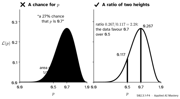
S02.3.1-F4

Wrong beside right. The likelihood’s height at 0.7 is not the chance that \({p = 0.7}\): the curve does not even have area 1. What it does support is a comparison of two values by a ratio.

“The likelihood is the probability that the parameter takes this value.”

\(\mathcal{L}(p)\) is the probability of the data given \(p\), written \({P(\text{data} \mid p)}\). The probability of \(p\) given the data, \({P(p \mid \text{data})}\), is a different quantity, and getting it needs a prior belief about \(p\) and Bayes’ rule (course S04). The likelihood answers “how well does this value explain what I saw?”, and it does so only in comparison with other values.

“Taking the log changes the answer, because the curve looks completely different.”

The heights change, and so does the shape: the log curve plunges towards minus infinity at both ends, where the likelihood only sinks to 0. But the order of any two values is kept, because \(\ln\) is increasing. So the highest point is in the same place. This holds for any increasing function, which is also why multiplying by 120 or dividing by \(n\) is harmless.

“A computer can just multiply the probabilities.”

Not for real data. A product of thousands of numbers below 1 rounds to zero, as the code showed, and then every parameter looks equally bad. Statistical software and every machine-learning library work with sums of log-probabilities for this reason.

Check yourself

Recall

1. What is the likelihood of a parameter value, in one sentence?

Show answer

The probability (or density) of the observed data computed under that parameter value, read as a function of the parameter with the data held fixed.

2. Why may we maximise \(\ell(\theta)\) instead of \(\mathcal{L}(\theta)\)?

Show answer

Because \(\ln\) is increasing: a larger likelihood always has a larger log-likelihood, so both peak at the same \(\theta\).

3. What is the MLE of the chance of heads after \(k\) heads in \(n\) tosses?

Show answer

\({\hat{p} = k / n}\), the share of heads seen; 0.7 for 7 heads in 10.

4. How many times as probable are 7 heads in 10 tosses if \({p = 0.7}\) as if \({p = 0.5}\)?

Show answer

\({0.7^7 \times 0.3^3 / 0.5^{10} = 2.28}\) times.

5. Does the area under the coin’s likelihood curve equal 1?

Show answer

No. With the factor 120 it is 1/11, and without it 1/1320. The likelihood is not a probability distribution over \(p\).

Exercises

1. ★ A classifier gets 90 of 100 test examples right. Treat each example as a toss with chance \(p\) of being right. Write the log-likelihood, find the MLE of \(p\), and compute \({\mathcal{L}(0.9) / \mathcal{L}(0.85)}\).

Show solution

\({\ell(p) = 90 \ln p + 10 \ln(1 - p)}\), and by the result above \({\hat{p} = 90/100 = 0.9}\). The log of the ratio is

\[ \begin{aligned} &90 \ln\tfrac{0.9}{0.85} + 10 \ln\tfrac{0.1}{0.15} \\ &\quad= 5.144 - 4.055 = 1.090, \end{aligned} \]

so the ratio is \({e^{1.090} \approx 2.97}\): the results are about three times as probable under 0.9 as under 0.85.

2. ★★ A coin shows 0 heads in 5 tosses. Write \(\mathcal{L}(p)\), explain why setting \({\ell'(p) = 0}\) finds nothing, and find the MLE.

Show solution

\({\mathcal{L}(p) = (1 - p)^5}\) and \({\ell'(p) = -5/(1 - p)}\), which is never zero: the curve falls all the way from \({p = 0}\) to \({p = 1}\). The largest value is at the left end, \({\mathcal{L}(0) = 1}\), so \({\hat{p} = 0 = 0/5}\). The formula \(k/n\) still holds, but the peak sits on the edge of the allowed range, where calculus’s flat-point test does not apply. Lesson S02.3.2 meets an edge peak again.

3. ★★★ Ten tosses come in two batches: 3 heads in the first 4 tosses and 4 heads in the last 6. Show that the log-likelihood of all ten is the sum of the two batches’ log-likelihoods, and that the MLE from all ten is not the average of the two batches’ MLEs.

Show solution

The batches are independent, so the likelihood of all ten is the product of the two batches’ likelihoods, and its log is the sum:

\[ \begin{aligned} &\big[3 \ln p + \ln(1 - p)\big] \\ &\quad + \big[4 \ln p + 2 \ln(1 - p)\big] \\ &\quad = 7 \ln p + 3 \ln(1 - p). \end{aligned} \]

That is the coin’s log-likelihood, with MLE \({7/10 = 0.7}\). The batch MLEs are \({3/4 = 0.75}\) and \({4/6 \approx 0.667}\), whose plain average is about 0.708. The pooled estimate weights each batch by its number of tosses: \({(4 \times 0.75 + 6 \times 0.667)/10 = 0.7}\).

Summary card

Fix the data and let the parameter vary: the top of the curve is the estimate.

The anchor figure again: on the left, binomial bars for 0 to 10 heads when p is 0.7, with the bar at 7 heads dark at 0.267; on the right, the likelihood of 7 heads as a vermillion hump over p, peaking at 0.267 at p equals 0.7. — S02.3.1-F1
One formula, two readings.

Likelihood. \(\mathcal{L}(\theta)\): the probability of the data, as a function of \(\theta\).
Log-likelihood. \({\ell = \ln \mathcal{L}}\): a sum over observations, same peak.
Coin. \(k\) heads in \(n\) tosses give \({\hat{p} = k/n}\).
Compare values by a ratio. \({\mathcal{L}(0.7)/\mathcal{L}(0.5) = 2.28}\).

Sources and next steps

Sources. Each was opened and checked against this lesson on 15 November 2026.

Jeremy Orloff and Jonathan Bloom, Reading 10b: Maximum Likelihood Estimates, MIT OpenCourseWare 18.05, Spring 2022. Section 3 defines the likelihood \({P(\text{data} \mid p)}\) and the MLE, works 55 heads in 100 tosses to the share of heads, warns against confusing \({P(\text{data} \mid p)}\) with \({P(p \mid \text{data})}\), and checks the maximum; Section 3.1 uses the log-likelihood.
Hossein Pishro-Nik, Introduction to Probability, Statistics, and Random Processes, Section 8.2.3: the likelihood as the joint probability mass function (or density) of the observed sample, read as a function of the parameter, the log-likelihood, and the binomial MLE.
NumPy documentation, numpy.argmax: returns the index of the largest value, the first one in case of ties, which is why an underflowed grid of zeros returns its first point.

Next. S02.3.2 Maximum likelihood for the standard families turns this into a recipe and runs it on counts, waiting times and serial numbers.

This lesson unlocks

S02.3.2 Maximum likelihood for the standard families

Your progress is saved in this browser only. No account, no tracking.