Compare several group means with one test: split the total sum of squares into a part between groups and a part within them, divide each by its degrees of freedom, and read their ratio F against the F distribution. Worked on rent by district and on the iris flowers.
S02.7.3L2 Intermediate25 minIn review (what this means)
The maths and code on this page are checked by automated tests on every change, but an independent reader has not signed it off yet. Spot a mistake or a confusing step? Tell us.
Derive the split of the total sum of squares into between-group and within-group parts, and compute both by hand.
Form the F statistic from the two mean squares and read its p-value from the F distribution with k - 1 and N - k degrees of freedom.
Show that for two groups the F statistic is the square of the pooled t statistic.
State the assumptions of one-way ANOVA and explain how a single outlier weakens it.
The question
The nine flats of S01 rent for a mean of 5 in the South, 8 in the North and 17 in the Centre (hundreds of euros). Three groups means three pairs to compare, and three t-tests each at level 0.05 give more than a 5 percent chance of a false alarm. Is there one test that asks “do these means differ at all?” There is, and machine learning uses it to screen thousands of features against a class label in one line.
From the last lesson
1. How are the expected counts of a two-way table found under independence?
Show answer
Row total times column total over the grand total, \({E_{gj} = n_{g\cdot} n_{\cdot j}/n}\); for South with a balcony, \({60 \times 60/120} = 30\).
2. Why does McNemar’s test use only 15 of the 100 test examples?
Show answer
Only the examples on which the two classifiers disagree carry information about which is better; under \(H_0\) each disagreement is a fair coin.
Intuition
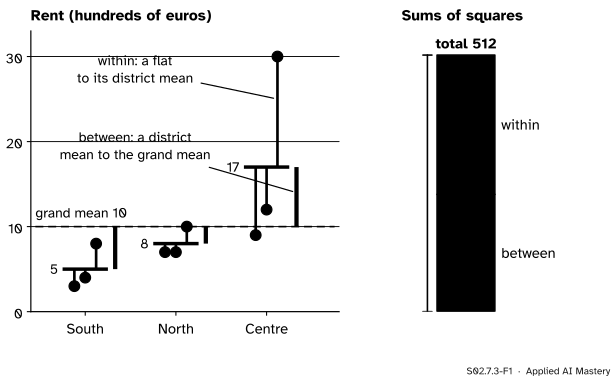
Measure how spread out all nine rents are, then ask where that spread comes from. Part of it is between the districts: their means differ. The rest is within them: flats in one district still differ from each other. If the districts truly had the same mean, the between part would be no bigger than the noise the within part shows.
S02.7.3-F1
Rent by district for the nine flats of S01 (invented). The total sum of squares, 512, splits exactly into 234 between the districts and 278 within them.
Here the within part is larger than the between part. That alone does not settle it, because the two parts rest on different numbers of free values: they are compared per degree of freedom. The comparison is the F statistic, and the method is the analysis of variance, ANOVA.
Build it up
Step 1. The total. Square each rent’s gap to the grand mean 10 and add: the total sum of squares, 512, the figure S01 computed.
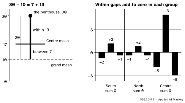
Step 2. Split each gap in two. Every flat’s gap to the grand mean is its district’s gap plus its own gap within the district. For the penthouse, \({30 - 10} = {(17 - 10) + (30 - 17)} = 7 + 13\).
S02.7.3-F5
Left: one flat’s gap split into a between part and a within part. Right: inside every group the within gaps cancel, which is what makes the squares add up.
Step 3. Square and add. Squares do not usually add: \({20^2 = 400}\) but \({7^2 + 13^2 = 218}\). Summed over a whole group, though, the cross terms cancel, because the within gaps of a group add to zero. So the sums of squares do add: \({234 + 278 = 512}\).
Step 4. Compare per degree of freedom. Three group means around one grand mean leave 2 free values; nine flats around three group means leave 6. Divide: \({234/2} = 117\) and \({278/6} = 46.33\). Their ratio is \(F = 2.53\).
The formal statement
Write \(k\) groups, \(n_g\) values \(x_{gi}\) in group \(g\), \(N = {\sum_g n_g}\) values in all, group means \(\bar x_g\) and grand mean \(\bar x\).
The mean squares are \({MS_B = SS_B/(k - 1)}\) and \({MS_W = SS_W/(N - k)}\), and \(F = {MS_B / MS_W}\). If the groups are independent normal samples with one variance and equal means, \(F\) follows the F distribution \(F_{k-1,\,N-k}\). The p-value is \({\Prob(F_{k-1,N-k} \ge F)}\).
The split, derived. Write each gap as a between part plus a within part and square:
Sum over \(i\) inside group \(g\). The first term does not depend on \(i\), so it gives \({n_g (\bar x_g - \bar x)^2}\). In the middle term the factor \({(\bar x_g - \bar x)}\) comes out of the sum, leaving \({\sum_i (x_{gi} - \bar x_g)} = {n_g \bar x_g - n_g \bar x_g} = 0\). Now sum over \(g\): \(SS_T = SS_B + SS_W\). The degrees of freedom split the same way: \({N - 1} = {(k - 1) + (N - k)}\).
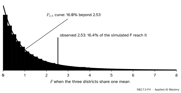
The F distribution. If \(U_1 \sim \chi^2_{\nu_1}\) and \(U_2 \sim \chi^2_{\nu_2}\) are independent, the ratio \({(U_1/\nu_1) / (U_2/\nu_2)}\) has the F distribution\(F_{\nu_1, \nu_2}\). In ANOVA, \({SS_W/\sigma^2}\) is a sum of the independent \({(n_g - 1)s_g^2/\sigma^2}\), each \(\chi^2_{n_g - 1}\) (S02.1.4), so it is \(\chi^2_{N-k}\); under \(H_0\), \({SS_B/\sigma^2}\) is \(\chi^2_{k-1}\) and independent of it (stated). The unknown \(\sigma^2\) cancels in the ratio. With \(k - 1 = 2\) the tail has a closed form, \({\Prob(F_{2,\nu} \ge f)} = {(1 + 2f/\nu)^{-\nu/2}}\); for the flats, \({(1 + 2 \times 2.53/6)^{-3}} = 0.160\).
S02.7.3-F4
When the three districts share one mean, F follows \(F_{2,6}\) exactly (black). In 20,000 simulated sets of nine normal rents (seed 2), 16.4 percent reach the observed 2.53, against 16.0 percent under the curve.
For two groups, \(F = t^2\). Let \(D = {\bar x_B - \bar x_A}\). The grand mean is \({(n_A \bar x_A + n_B \bar x_B)/N}\), so \({\bar x_A - \bar x} = -n_B D/N\) and \({\bar x_B - \bar x} = n_A D/N\). Then
With \(k = 2\), \(MS_B = SS_B\), and \(MS_W\) is the pooled variance of S02.7.1, so \({F = D^2 / (s_{\text{pool}}^2 (1/n_A + 1/n_B))} = t^2\). For the two designs, \(F = 3\) and \(t = \sqrt 3\), with the same p-value 0.122.
Assumptions. Independent observations, a normal population in each group, and one shared variance. The flats break the last two: Centre’s standard deviation is 11.4 against 2.6 and 1.7, all because of the penthouse. Lower the penthouse to 15 and \(F\) rises to 5.84, p-value 0.039; raise it to 60 and \(F\) falls to 1.55, p-value 0.29. A more extreme Centre flat makes the test less sure the Centre differs, because the flat inflates the within part more than the between part.
Worked example
Do the three districts differ in mean rent? South 3, 8, 4; North 7, 10, 7; Centre 12, 30, 9.
S02.7.3-F2
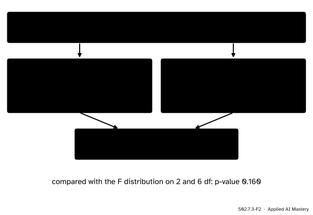
One-way ANOVA on the nine flats, from the means to the p-value.
Means: South \({15/3} = 5\), North \({24/3} = 8\), Centre \({51/3} = 17\); grand mean \({90/9} = 10\).
Between: each group has 3 flats, so \(SS_B\) is 3 times the sum of the squared gaps of the district means, \({(5 - 10)^2} = 25\), \({(8 - 10)^2} = 4\) and \({(17 - 10)^2} = 49\): \({3 \times 78} = 234\).
Within. South: \({4 + 9 + 1} = 14\). North: \({1 + 4 + 1} = 6\). Centre: \({25 + 169 + 64} = 258\). So \(SS_W = 278\), and \(234 + 278 = 512\) checks against the total.
Mean squares: \({234/2} = 117\) and \({278/6} = 46.33\). \(F = 2.53\) on 2 and 6 degrees of freedom.
At level 0.05 the test does not reject equal means. With three flats per district and one penthouse, it cannot tell the districts apart, even though the Centre mean is more than three times the South mean.
Code
From scratch, then a simulation of \(F\) under \(H_0\).
import numpy as npfrom scipy import statsgroups = {"South": [3, 8, 4], "North": [7, 10, 7], "Centre": [12, 30, 9]} # S01's flats (invented)def anova(groups): arrays = [np.asarray(v, dtype=float) for v in groups] every = np.concatenate(arrays) grand = every.mean() ss_b =sum(len(a) * (a.mean() - grand) **2for a in arrays) ss_w =sum(((a - a.mean()) **2).sum() for a in arrays) k, n =len(arrays), len(every) f = (ss_b / (k -1)) / (ss_w / (n - k))return ss_b, ss_w, f, stats.f.sf(f, k -1, n - k)ss_b, ss_w, f, p = anova(groups.values())print(ss_b, ss_w, ss_b + ss_w, round(f, 3), round(p, 3), "closed form:", (1+2* f /6) **-3)rng = np.random.default_rng(2)sims = rng.normal(0, 1, size=(20_000, 3, 3)) # 3 groups of 3, one shared meanmeans = sims.mean(axis=2)f_sim = (3* ((means - sims.mean(axis=(1, 2))[:, None]) **2).sum(axis=1) /2) \/ (((sims - means[:, :, None]) **2).sum(axis=(1, 2)) /6)print("simulated share reaching 2.53:", np.mean(f_sim >= f))
The library call, then the iris flowers as a real case: petal length by species, and f_classif, which computes the same F for every feature column against a class label.
from sklearn.datasets import load_irisfrom sklearn.feature_selection import f_classifres = stats.f_oneway(*groups.values())print(res.statistic, res.pvalue)iris = load_iris()petal = iris.data[:, 2]by_species = [petal[iris.target == k] for k inrange(3)]print("petal length:", stats.f_oneway(*by_species))f_all, p_all = f_classif(iris.data, iris.target)print(dict(zip(iris.feature_names, np.round(f_all, 1))))
Petal length gives \(F = 1180\) with 2 and 147 degrees of freedom: the species means 1.46, 4.26 and 5.55 cm are far apart compared with the spread inside each species. Feature screening with SelectKBest(f_classif) keeps the columns with the largest such F.
Explore
S02.7-X1
ANOVA decomposer
Drag any flat up or down, or choose it and use the slider or the minus and plus buttons. Add or remove flats in a district. The bar splits the total sum of squares into between and within, and the read-out gives \(F\) and its p-value. Press Ranks to replace each rent by its rank.
Things to try. Drag the penthouse from 30 up to 60 and then down to 13: \(F\) rises as it comes down, and the p-value crosses 0.05 between 16 and 17. Watch \(H\), the Kruskal-Wallis statistic of S02.7.4, in the read-out as you drag: as long as the penthouse stays the highest rent its rank is 9, so \(H\) does not move. Press Ranks to see why: there the flats are moved with the slider or the buttons, and the penthouse’s dot stays at rank 9. Finally make every district’s flats equal: the within part is 0 and \(F\) has no finite value.
Pitfalls
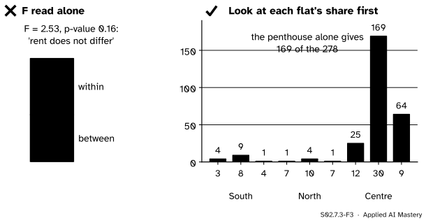
S02.7.3-F3
Wrong beside right. One F value hides that a single flat supplies most of the within-group spread.
“p-value 0.16, so rent does not differ between districts.”
A large p-value means these nine flats cannot show a difference, not that there is none. Here one flat supplies 169 of the 278 within-group units, the equal-variance assumption fails, and the groups hold three flats each. Plot the groups first, and consider the rank test of S02.7.4.
“F is significant, so every district differs from every other.”
ANOVA asks one question: are all the means equal? A small p-value says at least one differs, not which. Comparing pairs afterwards needs a correction for the several tests, such as Tukey’s method in S02.9.4.
“Three t-tests do the same job as one ANOVA.”
Three tests at level 0.05 each give a family-wise false-alarm chance above 0.05 (S02.9.1). ANOVA spends 0.05 once on the overall question.
Check yourself
Recall
1. What are the between-group and within-group sums of squares for rent by district, and what do they add to?
Show answer
234 and 278, adding to the total 512.
2. Why does \(SS_T = SS_B + SS_W\) hold, when squares do not usually add?
Show answer
The cross term \({2(\bar x_g - \bar x)\sum_i (x_{gi} - \bar x_g)}\) is zero in every group, because the within gaps of a group add to zero.
3. Give \(F\), its degrees of freedom and the p-value for the flats.
Show answer
\({F = 117/46.33} = 2.53\) on 2 and 6 degrees of freedom, p-value 0.160.
4. What is the F distribution?
Show answer
The distribution of \({(U_1/\nu_1)/(U_2/\nu_2)}\) for independent \(U_1 \sim \chi^2_{\nu_1}\) and \(U_2 \sim \chi^2_{\nu_2}\).
5. How are ANOVA’s \(F\) and the pooled two-sample \(t\) related for two groups?
Show answer
\(F = t^2\), with the same p-value: for the two designs \(F = 3\) and \(t = \sqrt 3\).
Exercises
1.★ Three groups of two: (2, 4), (5, 7) and (8, 12). Compute \(SS_B\), \(SS_W\), \(F\) and the p-value.
Show solution
Means 3, 6 and 10; grand mean \({38/6} = 6.33\). Between:
Within: \({14 + 6 + 18} = 38\). So \({F = (74/2)/(38/6)} = 5.84\) and the p-value is \({(1 + 2 \times 5.84/6)^{-3}} = 0.039\). The between part shrank from 234 to 74, but the within part shrank far more, from 278 to 38, so the ratio grew.
3.★★★ Suppose \(H_0\) holds and every group has \(m\) values from a population with variance \(\sigma^2\). Show that \(\E[MS_W] = \sigma^2\) and \(\E[MS_B] = \sigma^2\), so \(F\) should be near 1 under \(H_0\).
Show solution
Within: \(MS_W = {\sum_g (m - 1)s_g^2 / (k(m - 1))}\) is the average of the \(k\) group variances, and each \(s_g^2\) is unbiased for \(\sigma^2\) (S02.2.1), so \(\E[MS_W] = \sigma^2\).
\(m\) times the sample variance of the \(k\) group means. Under \(H_0\) the group means are independent with common mean \(\mu\) and variance \(\sigma^2/m\), so their sample variance has expectation \(\sigma^2/m\) (S02.2.1 again). Hence \({\E[MS_B] = m \cdot \sigma^2/m} = \sigma^2\). When the true means differ, the group means spread out more and \(MS_B\) grows, while \(MS_W\) does not.
Summary card
Split the spread into between and within, and compare them per degree of freedom.
Statistic.\(F = {MS_B / MS_W}\), compared with \(F_{k-1,\,N-k}\).
Two groups.\(F = t^2\).
Assumptions. Independence, normality, one shared variance; outliers inflate \(SS_W\).
Sources and next steps
Sources. Each was opened and checked against this lesson on 15 November 2026.
MIT OpenCourseWare 18.05, Reading 19, Null Hypothesis Significance Testing III, Spring 2022 (free PDF). Section 4.4 gives one-way ANOVA with equal group sizes: the assumptions, \(MS_B\) as \(m\) times the sample variance of the group means, \(MS_W\) as the average group variance, and the null distribution \({F(n - 1, n(m - 1))}\).
SciPy developers, scipy.stats.f_oneway (assumptions: independent samples, normal populations, equal standard deviations, with the Kruskal-Wallis test as an alternative) and scipy.stats.f (the ratio of two independent chi-squared variables, with shape parameters dfn and dfd).
Next.S02.7.4 Rank tests replaces values by ranks, which the penthouse cannot pull. Comparisons between pairs of districts after an ANOVA are in S02.9.4.