Power is the chance that a test notices an effect that is really there. Derive it for the one-sided z-test from the overlap diagram, read off what raises it, draw the power curve, and check the formula by simulation on the city’s rents.
S02.6.1L2 Intermediate25 minIn review (what this means)
The maths and code on this page are checked by automated tests on every change, but an independent reader has not signed it off yet. Spot a mistake or a confusing step? Tell us.
Define power as 1 − β, the probability of rejecting the null hypothesis when a stated alternative is true, and point to it on the overlap diagram.
Derive the power of the one-sided z-test from the overlap diagram and compute it by hand.
Read off the power formula how a larger effect, a larger sample, a smaller σ, a larger α and a one-sided test each raise power.
Draw and interpret the power curve against the true effect and against the sample size.
Check a power calculation by a seeded simulation.
The question
Last year the mean rent in the city of S01 was 8.3 hundred euros a month. A housing office will sample 25 flats this year and run a one-sided z-test at level 0.05 for a rise. Suppose the mean really has risen, by 2 to 10.3. How likely is the test to notice? The answer, 0.58, is barely better than a coin toss, and the same arithmetic decides whether a test set can show that a new model beats an old one.
Intuition
Lesson S02.5.3 drew two sampling distributions of the test statistic: one if the null hypothesis \(H_0\) is true, one if a particular alternative \(H_1\) is true, with the critical value between them. This lesson calls it the cut-off. Power lives on the second curve.
S02.6.1-F1
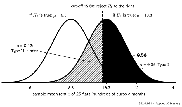
The overlap diagram for the rent test with 25 flats. If the mean has risen to 10.3, the sample mean is drawn from the sky-blue curve. It lands beyond the cut-off, and the test rejects \(H_0\), with probability 0.58: the power. The hatched area is the chance of a miss, \(\beta\).
Read the picture as a story about one study that has not happened yet. If the true mean is 10.3, the sample mean will fall somewhere under the sky-blue curve. Wherever it falls to the right of the orange cut-off, the test says “the rent has risen” and is right. Wherever it falls to the left, the test says “no evidence of a rise” and misses a rise that is real.
The power of a test against an alternative is the probability that the test rejects \(H_0\) when that alternative is true. It is the green area. The hatched area is the Type II error rate \(\beta\), so power is \(1 - \beta\). The solid sliver under the black curve is \(\alpha\): it was fixed in advance, and it is what placed the cut-off where it is.
Build it up
Step 1. The null curve fixes the cut-off. Treat \(\sigma = 5.41\) as known (it is the city’s spread). With \(n = 25\) flats the standard error of \(\bar{x}\) is \({5.41/\sqrt{25}} = 1.082\) (S02.1.2). If \(H_0\) is true, \(\bar{x}\) is close to normal with mean 8.3 and standard deviation 1.082. The one-sided test at level 0.05 rejects when \(\bar{x}\) is more than \(z_{0.95} = 1.645\) standard errors above 8.3, that is when \(\bar{x} > 10.08\).
Step 2. The alternative moves the same bell. If the true mean is 10.3, \(\bar{x}\) has the same spread, 1.082, but is centred at 10.3. Nothing about the cut-off changes: the test does not know which curve the data came from.
Step 3. Power is an area. The power is the area under the moved bell to the right of 10.08. The cut-off sits \({0.22/1.082} = 0.20\) standard errors to the left of 10.3, so a little more than half of the bell is beyond it: 0.58.
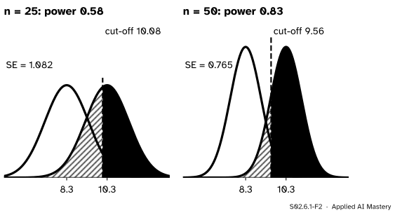
Step 4. More data narrows both bells. Double the sample to 50 flats. The standard error falls to \({5.41/\sqrt{50}} = 0.765\), the cut-off comes in to 9.56, and the two bells overlap less.
S02.6.1-F2
The same rise of 2 with 25 flats and with 50. The bells narrow by a factor \(\sqrt{2}\), the cut-off moves towards 8.3, and the power climbs from 0.58 to 0.83.
The gap between the centres is the same 2 in both panels. What changed is the ruler: measured in standard errors, the gap grew from 1.85 to 2.61.
The formal statement
NoteDefinition: power
For a test of \(H_0\) at level \(\alpha\) and a particular value \(\theta_1\) of the parameter allowed by \(H_1\),
Seen as a function of the true value, it is the power function of the test.
The one-sided z-test. Take \(n\) independent draws with known \(\sigma\), \(H_0: \mu = \mu_0\) against \(H_1: \mu > \mu_0\). The statistic is \({Z = (\bar{X} - \mu_0)/(\sigma/\sqrt{n})}\), and the test rejects when \(Z \ge z_{1-\alpha}\). Suppose the true mean is \(\mu_0 + \Delta\) with \(\Delta > 0\). Then \(\bar{X}\) has mean \(\mu_0 + \Delta\) and standard deviation \({\sigma/\sqrt{n}}\), exactly for normal data and approximately for large \(n\) by the central limit theorem (M06.11.3). Split \(Z\) into a standard normal part and a shift:
where \(Z'\) is standard normal under the alternative. So \(Z\) is a standard normal moved right by \(\lambda = {\Delta\sqrt{n}/\sigma}\), the gap measured in standard errors. The power is
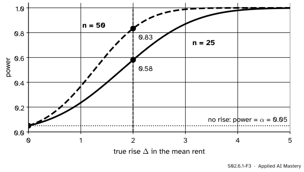
At \(\Delta = 0\) this is \({1 - \Phi(z_{1-\alpha})} = \alpha\): with no effect, the test rejects exactly as often as its level allows. As \(\Delta\) grows, the argument of \(\Phi\) falls and the power climbs towards 1.
S02.6.1-F3
The power function of the one-sided rent test. Every curve starts at \(\alpha\) when there is no effect. A larger sample makes the curve rise sooner.
What raises power. Every lever is in the one formula. Power grows when the argument \({z_{1-\alpha} - \lambda}\) falls, so when \(\lambda = {\Delta\sqrt{n}/\sigma}\) grows or \(z_{1-\alpha}\) shrinks. For the rent test (power 0.58 at the start):
Change
What moves
Power
rise 2 → 3
\(\lambda\) 1.85 → 2.77
0.87
\(n\) 25 → 50
\(\lambda\) 1.85 → 2.61
0.83
\(\sigma\) 5.41 → 4
\(\lambda\) 1.85 → 2.50
0.80
\(\alpha\) 0.05 → 0.10
\(z\) 1.645 → 1.282
0.71
A two-sided test at the same level puts its cut-off at \(z_{0.975} = 1.96\) instead of 1.645, so it has less power against a rise: it is also watching for a fall. Its power picks up a second, tiny tail on the far side,
Two groups. To compare two groups of \(n\) each, the statistic is the difference \({\bar{X}_B - \bar{X}_A}\). Its variance is the sum of the two variances (S02.4.4), so its standard error is \({\sigma\sqrt{2/n}}\) and the shift becomes
The standardised effect \(\delta\) is the subject of the next lesson. The module’s interactive uses this two-group form.
Go deeper: why the z-test answer is only approximate for real rents
The derivation used one fact: that \(\bar{X}\) is normal with standard deviation \({\sigma/\sqrt{n}}\). For the city’s skewed rents that is only roughly true at \(n = 25\). Their skewness is about 1.76, so the skewness of \(\bar{X}\) is about \({1.76/\sqrt{25}} = 0.35\) (S02.1.3), and the right tail of \(\bar{X}\) is a little longer than the normal’s while most of its mass sits slightly to the left. The code below simulates the test on the real rents and finds a power of about 0.56 instead of 0.58. When the distribution matters, simulate: lesson S02.6.4 makes that the general method.
Worked example
The rent test, by hand.\(\mu_0 = 8.3\), \(\sigma = 5.41\), \(n = 25\), \(\alpha = 0.05\) one-sided, and the alternative to detect is a rise of \(\Delta = 2\).
S02.6.1-F4
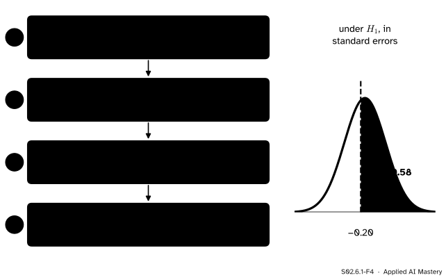
The four steps of a power calculation. The last step reads a normal area, the green part of the alternative’s curve measured in standard errors.
The standard error is \({5.41/\sqrt{25}} = 1.082\).
The cut-off is \({8.3 + 1.645 \times 1.082} = 10.08\).
Under the alternative, \(\bar{x}\) is centred at 10.3, so the cut-off is \({(10.08 - 10.3)/1.082} = -0.20\) standard errors from that centre.
The power is \({1 - \Phi(-0.20)} = \Phi(0.20) = 0.58\), and \(\beta = 0.42\).
The formula gives the same in one line: \({\lambda = 2 \times 5/5.41} = 1.848\), and \({1 - \Phi(1.645 - 1.848)} = 0.58\). A two-sided test at level 0.05 would have power \({1 - \Phi(1.960 - 1.848)} + \Phi(-3.808) = 0.46\).
So a study of 25 flats misses a real rise of 200 euros a month 42 times in 100. That is the answer to the question, and it should worry the housing office before it samples a single flat.
Code
From scratch first: \(\Phi\) from math.erf, and the quantile \(z_{0.95}\) from the standard library’s statistics.NormalDist.
import mathfrom statistics import NormalDistdef Phi(x):"""The standard normal cumulative distribution function."""return0.5* (1+ math.erf(x / math.sqrt(2)))def z_power(delta, n, sigma, alpha=0.05, two_sided=False):"""Power of the z-test against a true shift `delta` of the mean.""" lam = delta * math.sqrt(n) / sigmaif two_sided: z = NormalDist().inv_cdf(1- alpha /2)return1- Phi(z - lam) + Phi(-z - lam)return1- Phi(NormalDist().inv_cdf(1- alpha) - lam)mu0, sigma, n =8.3, 5.41, 25se = sigma / math.sqrt(n)cut = mu0 + NormalDist().inv_cdf(0.95) * seprint(f"SE {se:.3f}, cut-off {cut:.2f}")print(f"power one-sided {z_power(2, 25, sigma):.3f}, two-sided {z_power(2, 25, sigma, two_sided=True):.3f}")for size in (10, 25, 50, 100):print(f"n = {size:3d}: power {z_power(2, size, sigma):.3f}")
SE 1.082, cut-off 10.08
power one-sided 0.581, two-sided 0.456
n =  10: power 0.317
n =  25: power 0.581
n =  50: power 0.834
n = 100: power 0.980
Now check by simulation. Draw 20,000 samples of 25 from a normal population with mean 10.3, run the test on each, and count rejections. Then do the same on the city’s own skewed rents, each raised by 2.
import numpy as nprng = np.random.default_rng(1)means = rng.normal(10.3, sigma, size=(20_000, 25)).mean(axis=1)sim_normal = np.mean((means - mu0) / se >1.6449)print("normal population: rejected", sim_normal)# the city of S01: 500 rents, built exactly as S01 builds themrng = np.random.default_rng(0)rents = []for mean, size in ((5, 250), (8, 150), (17, 100)): draws = rng.gamma(9.0, 1.0, size) rents.append(draws * mean / draws.mean())city = np.concatenate(rents)rng = np.random.default_rng(2)means = rng.choice(city +2, size=(20_000, 25)).mean(axis=1)print("city rents raised by 2: rejected", np.mean((means - mu0) / se >1.6449))
normal population: rejected 0.57685
city rents raised by 2: rejected 0.5579
The normal population gives about 0.58, as the formula says. The skewed rents give about 0.56: the formula is a good guide, and the simulation is the check. The library version is one line, scipy.stats.norm.sf(z - lam):
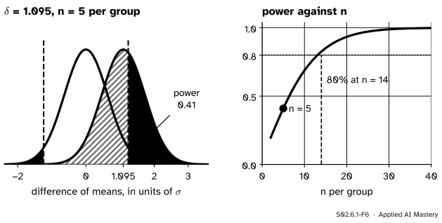
Set the standardised effect\(\delta\), the sample size per group, the level α and one- or two-sided. Watch the alternative’s bell slide away from the null’s as \(\delta\) or \(n\) grows, and read the \(n\) needed for 80 percent power off the curve on the right.
It opens on the two page designs of S02.4.4: \(\delta = 1.095\) and five visitors per group, the case of the next two lessons. Things to notice: at \(\delta = 0\) the power is \(\alpha\) whatever \(n\) is; halving \(\delta\) roughly quadruples the \(n\) needed; and switching to one-sided moves one cut-off inwards and deletes the other. The explorer uses the normal approximation, so its powers are a little higher than the exact t-test’s (lesson S02.6.3).
Pitfalls
S02.6.1-F5
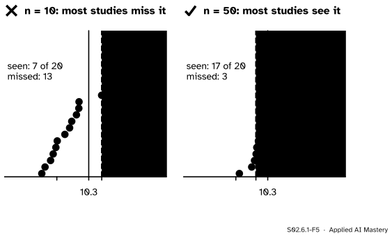
Twenty imagined studies of the same real rise. With 10 flats each, most of them miss it (power 0.32). With 50 each, most of them see it (power 0.83).
“The test was not significant, so the rent has not risen.”
A test with power 0.32 misses a real rise of 2 about two times in three. “Not significant” means the data are compatible with no rise; it does not show there was none. Before reading a null result, ask what power the study had against an effect that would matter.
“This test has power 0.8.”
Power is not one number. It is a function of the true effect, and also of \(\sigma\), \(n\) and \(\alpha\). “Power 0.8 to detect a rise of 2 with 50 flats at level 0.05” is a statement; “power 0.8” alone is not.
“Power is the probability that the alternative is true.”
Power is computed assuming a particular alternative is true. It says how often the test would catch that effect, not how likely the effect is.
“For more power, just raise α.”
It works (0.58 becomes 0.71 at level 0.10), but every bit of it is paid for with false alarms when there is no effect. Sample size and a cleaner measurement buy power without that price. The same trade appears when a classifier’s threshold is moved (ML01.6.4).
Check yourself
Recall
1. Define the power of a test against a particular alternative.
Show answer
The probability that the test rejects \(H_0\) when that alternative is true, \(1 - \beta\).
2. On the overlap diagram, which area is the power?
Show answer
The area under the alternative’s curve on the rejecting side of the cut-off.
3. Write the power of the one-sided z-test against a rise \(\Delta\).
4. What is the power when \(\Delta = 0\), and why?
Show answer
\(\alpha\), because then the alternative’s curve is the null’s curve, and the area beyond the cut-off is exactly the level.
5. Name four changes that raise power.
Show answer
A larger true effect, a larger sample, a smaller \(\sigma\), a larger \(\alpha\) (and a one-sided test when the direction is known in advance).
Exercises
1.★ The housing office samples 100 flats instead of 25. Find the power of the one-sided level-0.05 test against a rise of 2.
Show solution
The standard error is \({5.41/\sqrt{100}} = 0.541\), so \({\lambda = 2/0.541} = 3.697\). The power is \({1 - \Phi(1.645 - 3.697)} = \Phi(2.052) = 0.98\).
2.★★ With 25 flats, the office decides to use a two-sided test at level 0.05. Compute its power against a rise of 2, and explain in one sentence why it is lower than 0.58.
Show solution
\(\lambda = 1.848\) as before. The power is \({1 - \Phi(1.960 - 1.848)} + \Phi(-1.960 - 1.848)\), which is \({0.4556 + 0.0001} = 0.46\). It is lower because the two-sided test splits its 0.05 between both tails, so its upper cut-off moves out from 1.645 to 1.96 standard errors, and the lower tail it gains is useless against a rise.
3.★★★ For the one-sided z-test, show that the power is above one half exactly when the true mean lies beyond the cut-off, and find the smallest rise the rent test detects with probability one half.
Show solution
Power is \({1 - \Phi(z_{1-\alpha} - \lambda)}\), which exceeds \(\tfrac12\) exactly when \({\Phi(z_{1-\alpha} - \lambda)} < \tfrac12\), that is when \({z_{1-\alpha} - \lambda} < 0\), because \(\Phi(0) = \tfrac12\) and \(\Phi\) is increasing. Multiply \({\lambda > z_{1-\alpha}}\) by \({\sigma/\sqrt{n}}\):
so \({\mu_0 + \Delta}\) is beyond the cut-off \({\mu_0 + z_{1-\alpha}\sigma/\sqrt{n}}\). For the rent test the half-power rise is \({1.645 \times 1.082} = 1.78\): a true mean of 10.08, right on the cut-off, is caught exactly half the time.
Summary card
Power is the chance of catching an effect that is really there.
Two groups of \(n\).\(\lambda = \delta\sqrt{n/2}\).
Levers. Larger \(\Delta\), \(n\) or \(\alpha\), smaller \(\sigma\), one-sided: more power.
Sources and next steps
Sources. Each was opened and checked against this lesson on 15 November 2026.
Jeremy Orloff and Jonathan Bloom, Reading 17b, Null Hypothesis Significance Testing I, MIT OpenCourseWare 18.05, Spring 2022. Section 4.3 defines power as P(reject \(H_0\) | \(H_A\)), one minus the probability of a Type II error; Section 4.4.2 draws high- and low-power tests as overlapping null and alternative curves with the power shaded.
David Diez, Mine Çetinkaya-Rundel and Christopher Barr, OpenIntro Statistics, 4th edition (free PDF). Section 7.4.2, “Computing the power for a 2-sample test”, finds the power of a two-group test as the area of the alternative’s distribution beyond the cut-offs, the method of the worked example here.
Next.S02.6.2 Effect size takes the \(\delta\) in \(\lambda = \delta\sqrt{n/2}\) and makes it a result to report in its own right.