Turn a bootstrap distribution into a confidence interval: the percentile interval, the basic interval derived from a pivot, and BCa, scipy’s default. Worked on the nine rents and on the diabetes correlation, with coverage checked on the city and the cases where the bootstrap fails.
S02.8.2L2 Intermediate25 minIn review (what this means)
The maths and code on this page are checked by automated tests on every change, but an independent reader has not signed it off yet. Spot a mistake or a confusing step? Tell us.
Compute the 95 percent percentile interval from the 2.5 and 97.5 percentiles of the replicates.
Derive the basic interval from the bootstrap version of the pivot, theta-hat minus theta, and compute it by hand.
Say what BCa corrects and call scipy.stats.bootstrap with method=‘percentile’, ‘basic’ and ‘BCa’, with paired=True for a correlation.
Check the coverage of bootstrap intervals by simulation, and name three cases where the bootstrap fails: the maximum, very small samples and dependent rows.
The question
In the diabetes table of S01.8, body mass index and the progression score have correlation 0.59 across 442 patients. A report should say how sure that number is. The intervals of S02.4 need a formula for the standard error, and the correlation has no simple one. How do we turn ten thousand resamples into an honest 95 percent interval, and when should we not trust it?
From the last lesson
1. Why does the bootstrap resample with replacement?
Show answer
Without replacement, \(n\) rows drawn from \(n\) are the same rows reordered, so every resample gives the same statistic. With replacement some rows repeat and others drop out, which mimics how a new sample would differ.
2. What does increasing the number of resamples \(K\) change, and what does it not change?
Show answer
It shrinks the Monte Carlo noise, so the estimate settles on the ideal bootstrap value. It does not shrink the standard error itself, which only more data (a larger \(n\)) can do.
Intuition
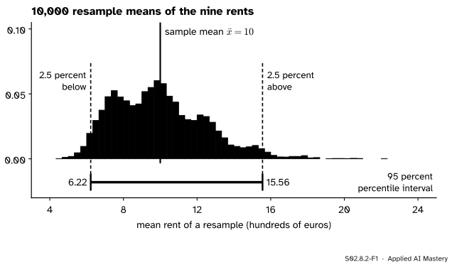
The bootstrap distribution shows where a statistic tends to land. Keep the middle 95 percent of it, cutting 2.5 percent off each end, and you have a range of plausible values: the percentile interval.
S02.8.2-F1
The percentile interval for the mean rent of the nine flats: the middle 95 percent of the 10,000 resample means. The distribution leans right, because resamples that catch the penthouse twice or three times have a large mean.
That is the whole recipe of the percentile interval, and it is often good. But the picture shows something to worry about: the distribution is lopsided, reaching 3.78 below the sample mean and 5.56 above it. Should the interval lean the same way as the bootstrap distribution, or the opposite way? The two simplest bootstrap intervals answer differently.
Build it up
Step 1. Name the cut points. Write \(q^*_p\) for the \(p\) quantile of the replicates: the value with a share \(p\) of them below it. For 95 percent we need \({q^*_{0.025} = 6.22}\) and \({q^*_{0.975} = 15.56}\).
Step 2. Read them directly. The percentile interval is \({[q^*_{0.025},\, q^*_{0.975}]}\): 6.22 to 15.56. It leans the same way as the bootstrap distribution.
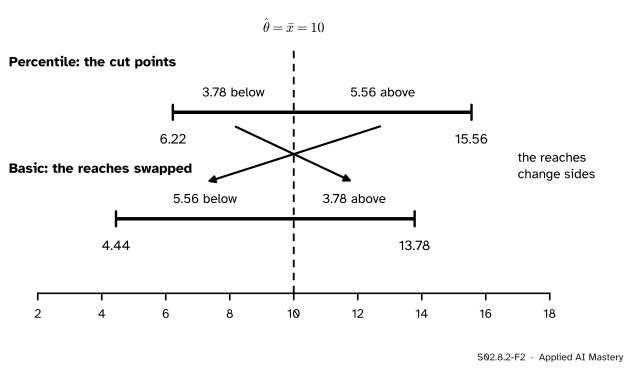
Step 3. Measure errors instead of values. What a confidence interval needs is the distribution of the error \({\hat\theta - \theta}\): how far the estimate tends to fall from the truth. The bootstrap world has its own error, \({\hat\theta^* - \hat\theta}\), the distance from a replicate to the sample’s value, playing the part of the truth. Its quantiles are the cut points minus 10: \({-3.78}\) and \({5.56}\).
Step 4. Undo the error. If the estimate tends to overshoot the truth by up to 5.56, then the truth can sit up to 5.56 below the estimate, and up to 3.78 above it. The reaches change sides: this is the basic interval, 4.44 to 13.78.
S02.8.2-F2
The basic interval is the percentile interval reflected about the estimate: the reach above becomes the reach below, and the other way round.
The formal statement
NoteDefinition: two bootstrap intervals
Let \(\hat\theta\) be the statistic of the sample and \(q^*_p\) the \(p\) quantile of the replicates \({\hat\theta^*_1, \dots, \hat\theta^*_K}\). The level \({1 - \alpha}\) percentile interval is
That is a confidence interval, the same pivot step as in S02.4.1. The \(d\)’s are unknown, so the plug-in principle replaces the error \({\hat\theta - \theta}\) by its bootstrap copy \({\hat\theta^* - \hat\theta}\), whose quantiles are \({q^*_p - \hat\theta}\). Substituting \({d_p \approx q^*_p - \hat\theta}\) into the two ends gives
The percentile interval has no such derivation; Hesterberg says it “just works”. Part of the reason is that it respects transformations: the percentile interval for \({\ln\theta}\) is the log of the percentile interval for \(\theta\), because taking logs keeps the replicates in order. Suppose some increasing transformation of \(\hat\theta\), which we need not know, makes the bootstrap distribution symmetric about the transformed estimate. On that scale the percentile and basic intervals coincide (exercise 2 below), and transforming back gives the percentile interval. So the percentile interval behaves like the basic interval on the best scale, without our having to find it.
BCa, the bias-corrected and accelerated interval, is scipy’s default. It still reads two percentiles of the replicates, but not the 2.5th and 97.5th. It shifts them using two estimates: the bias correction, from the share of replicates below \(\hat\theta\) (half of them, if the bootstrap distribution is centred on the estimate), and the acceleration, which allows for a standard error that changes with the parameter, one source of skewness. For a symmetric, unbiased case both corrections vanish and BCa is the percentile interval.
Go deeper: why the basic interval leans the wrong way for skewed data
The derivation assumes that \({\hat\theta - \theta}\) has the same distribution whatever \(\theta\) is, so that the bootstrap error \({\hat\theta^* - \hat\theta}\) can stand in for it. For a mean of skewed data this fails: samples with a high mean also have a high spread (the penthouse raises both), so the error distribution changes with where the sample happens to land. Hesterberg’s study finds that the basic interval is asymmetric in the wrong direction for skewed data and covers badly, and advises against using it in practice. BCa’s acceleration term is the correction designed for exactly this.
Worked example
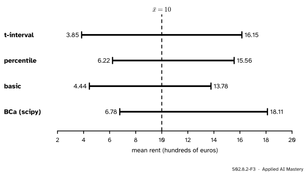
The mean rent of the nine flats. From lesson S02.8.1, \({\bar{x} = 10}\) and \({s = 8}\), and the code’s 10,000 resample means have \({q^*_{0.025} = 6.22}\) and \({q^*_{0.975} = 15.56}\). Each resample mean is a ninth of a sum of whole rents, so these are \({56/9}\) and \({140/9}\).
t-interval (S02.4.2), with \({t_{8,\,0.975} = 2.306}\): \({10 \pm 2.306 \times 8/3}\), that is 3.85 to 16.15.
BCa (scipy, 9,999 resamples): 6.78 to 18.11.
S02.8.2-F3
Four 95 percent intervals from the same nine rents. They disagree by several hundred euros at each end: nine skewed values hold too little information for any method to be sure.
The percentile and BCa intervals lean upwards, like the data; the basic interval leans downwards; the t-interval is symmetric by construction. With nine rents and a penthouse, the honest conclusion is that the mean rent is poorly pinned down, somewhere between about 4 and 18.
Code
From scratch for the nine rents, using the same 10,000 resamples as lesson S02.8.1:
import numpy as npfrom scipy import statsrents = np.array([7, 12, 3, 10, 30, 8, 9, 4, 7], dtype=float) # the nine flats of S01n, K =len(rents), 10_000rng = np.random.default_rng(0)means = rents[rng.integers(0, n, size=(K, n))].mean(axis=1)xbar = rents.mean()lo, hi = np.percentile(means, [2.5, 97.5])basic = (2* xbar - hi, 2* xbar - lo)half = stats.t.ppf(0.975, n -1) * rents.std(ddof=1) / np.sqrt(n)print(f"percentile {lo:.2f} to {hi:.2f}; basic {basic[0]:.2f} to {basic[1]:.2f}")print(f"t-interval {xbar - half:.2f} to {xbar + half:.2f}")
percentile 6.22 to 15.56; basic 4.44 to 13.78
t-interval 3.85 to 16.15
The diabetes correlation. A resample takes whole patients, so body mass index and score are drawn together, by one set of row numbers:
from sklearn.datasets import load_diabetestable = load_diabetes(as_frame=True, scaled=False).frame # 442 patients (S01.8)bmi, score = table["bmi"].to_numpy(float), table["target"].to_numpy(float)def corr(x, y, axis=-1): dx = x - x.mean(axis=axis, keepdims=True) dy = y - y.mean(axis=axis, keepdims=True)return (dx * dy).sum(axis=axis) / np.sqrt((dx **2).sum(axis=axis) * (dy **2).sum(axis=axis))r = corr(bmi, score)rows = np.random.default_rng(0).integers(0, len(score), size=(K, len(score)))reps = corr(bmi[rows], score[rows], axis=1)print(f"r = {r:.3f}; percentile interval {np.percentile(reps, 2.5):.3f} to {np.percentile(reps, 97.5):.3f}")for method in ("percentile", "basic", "BCa"): ci = stats.bootstrap((bmi, score), corr, paired=True, vectorized=True, method=method, rng=np.random.default_rng(0)).confidence_intervalprint(f"scipy {method:>10}: {ci.low:.3f} to {ci.high:.3f}")
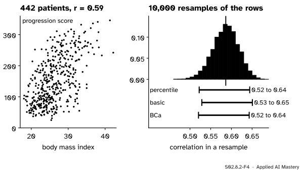
r = 0.586; percentile interval 0.522 to 0.644
scipy percentile: 0.522 to 0.644
scipy      basic: 0.529 to 0.651
scipy        BCa: 0.521 to 0.643
paired=True tells scipy to resample row numbers and apply them to both arrays, as our code did. With 442 patients the three methods agree to within 0.01: percentile and BCa 0.52 to 0.64, basic 0.53 to 0.65.
S02.8.2-F4
Resampling whole patients keeps each pair together. With 442 rows the bootstrap distribution of the correlation is nearly symmetric, and the three intervals almost coincide.
Does 95 percent mean 95 percent? On the city of S01 we know the truth, so we can draw a sample, build its interval, and count how often the interval covers the true value:
def city(): rng = np.random.default_rng(0) # the 500 flats, built exactly as in S01 parts = []for size, mean in ((250, 5), (150, 8), (100, 17)): draws = rng.gamma(9.0, 1.0, size) parts.append(draws * mean / draws.mean())return np.concatenate(parts)pop = city()def coverage(stat, n, truth, reps=1000, k=1000, seed=1): rng = np.random.default_rng(seed) hits =0for _ inrange(reps): x = rng.choice(pop, size=n) a, b = np.percentile(stat(x[rng.integers(0, n, size=(k, n))], axis=1), [2.5, 97.5]) hits += a <= truth <= breturn hits / repscover = {(name, m): coverage(f, m, f(pop)) for name, f in (("mean", np.mean), ("median", np.median))for m in (5, 25)}cover[("maximum", 25)] = coverage(np.max, 25, pop.max())print(cover)
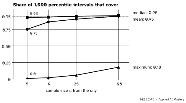
Percentile intervals for the mean cover only 75 percent of the time at \({n = 5}\) and 91 percent at \({n = 25}\): too narrow, as the factor \({\sqrt{(n-1)/n}}\) of the last lesson and the city’s skew predict. The median does better here, 93 and 95 percent.
Explore
The module’s resampling machine is in lesson S02.8.1. Draw a thousand resamples of the median and of the mean there and watch the percentile interval it marks: the median’s interval jumps between rents, the mean’s moves smoothly.
Pitfalls
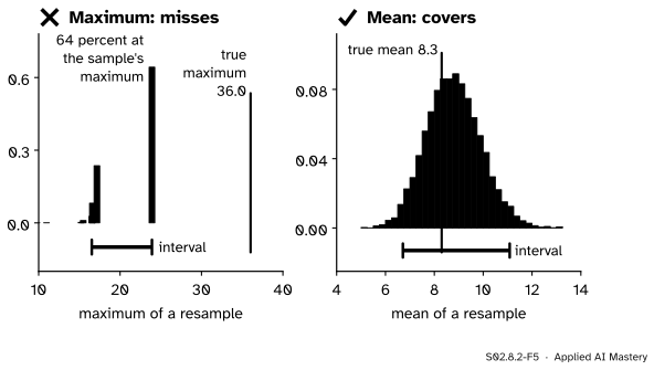
S02.8.2-F5
Wrong beside right, on one sample of 25 flats. A resample can never exceed the sample’s own maximum, so the interval for the maximum stops short of the truth.
“The bootstrap works for any statistic.”
It fails for the maximum. A resample’s maximum is the sample’s maximum unless that row is left out, so it equals it with probability \({1 - (1 - 1/n)^n}\), 0.64 for \({n = 25}\), and it can never be larger. The true maximum lies above every sample maximum unless the sample caught it, so the percentile interval covers it only 6 percent of the time at \({n = 25}\). Extremes, and statistics that hang on one or two rows, need other methods.
S02.8.2-F6
Coverage of 95 percent percentile intervals on the city. The mean needs a large sample before it earns its 95 percent; the maximum never does.
“Five numbers are enough, because the bootstrap needs no assumptions.”
The bootstrap assumes the sample is a good picture of the population, and five numbers are not. At \({n = 5}\) the percentile interval for the mean covers three times in four. Small samples give bootstrap distributions that are too narrow and too dependent on the few values drawn.
“Resample the rows of a time series like any other table.”
The bootstrap of this lesson assumes the rows are independent. Daily sales, sensor readings or the tokens of one document are not: resampling single rows breaks the dependence and gives intervals that are too narrow. Resampling blocks of neighbouring rows is the usual fix, a topic for the time-series course (S07).
Check yourself
Recall
1. How is the 95 percent percentile interval computed?
Show answer
From the 2.5th and 97.5th percentiles of the \(K\) replicates: \({[q^*_{0.025},\, q^*_{0.975}]}\).
2. What pivot does the basic interval come from, and what replaces it?
Show answer
The error \({\hat\theta - \theta}\); the bootstrap error \({\hat\theta^* - \hat\theta}\) stands in for it.
3. What are the two corrections in BCa?
Show answer
A bias correction, from the share of replicates below \(\hat\theta\), and an acceleration, for a standard error that changes with the parameter (skewness).
4. Why does scipy.stats.bootstrap need paired=True for a correlation?
Show answer
Because a resample must draw whole rows, keeping each patient’s two values together. Without it, scipy would resample each array on its own and destroy the pairing.
5. Name three cases where the bootstrap of this lesson fails.
Show answer
The maximum (or other extremes), very small samples, and dependent rows such as time series.
Exercises
1.★ A statistic is \({\hat\theta = 0.70}\) and its replicates have \({q^*_{0.025} = 0.62}\) and \({q^*_{0.975} = 0.75}\). Give the percentile and the basic 95 percent intervals.
Show solution
Percentile: 0.62 to 0.75. Basic: \({2 \times 0.70 - 0.75 = 0.65}\) to \({2 \times 0.70 - 0.62 = 0.78}\). The percentile interval reaches 0.08 below and 0.05 above; the basic interval swaps the reaches.
2.★★ Show that the percentile and basic intervals are the same whenever the bootstrap distribution is symmetric about \(\hat\theta\).
Show solution
Symmetry about \(\hat\theta\) means \({q^*_{1-p} - \hat\theta = \hat\theta - q^*_p}\) for every \(p\), that is \({q^*_{1-p} = 2\hat\theta - q^*_p}\). With \({p = \alpha/2}\) this says \({2\hat\theta - q^*_{\alpha/2} = q^*_{1-\alpha/2}}\), so the basic upper end equals the percentile upper end. With \({p = 1 - \alpha/2}\) it says \({2\hat\theta - q^*_{1-\alpha/2} = q^*_{\alpha/2}}\), so the lower ends agree too.
3.★★★ A sample of \({n = 25}\) values comes from a continuous population whose largest possible value is \(M\). Show that every bootstrap percentile interval for \(M\) lies below \(M\), and find the probability that the resample maximum equals the sample maximum.
Show solution
Every value of the sample is below \(M\), because the population is continuous, so a single value equals \(M\) with probability 0. A resample contains only sample values, so every replicate is at most the sample maximum, and so is every percentile of the replicates: the interval lies below \(M\) and never covers it. The resample maximum equals the sample maximum unless that one row is left out, which happens with probability \({(1 - 1/25)^{25} = 0.360}\), so the probability is \({1 - 0.360 = 0.640}\).
Summary card
Read an interval off the bootstrap distribution, and check that it covers.
BCa. Shifted percentiles, corrected for bias and skewness; scipy’s default.
Fails for maxima, tiny samples and dependent rows.
Sources and next steps
Sources. Each was opened and checked against this lesson on 15 November 2026.
Jeremy Orloff and Jonathan Bloom, Reading 24: Bootstrap confidence intervals, MIT OpenCourseWare 18.05, Spring 2022. Example 6 builds the percentile interval and the basic interval, which it also calls the reverse percentile interval, from the pivot \({\delta = \bar{x} - \mu}\) approximated by \({\delta^* = \bar{x}^* - \bar{x}}\).
Tim Hesterberg, What Teachers Should Know about the Bootstrap, arXiv:1411.5279 (2014). Section 4.1 shows that the percentile interval is transformation invariant; section 4.2 describes BCa’s bias estimate, the share of the bootstrap distribution at or below \(\hat\theta\); section 5.2 finds the percentile interval too narrow in small samples; section 5.4 says the percentile interval has no particular derivation, derives the reverse percentile interval, finds it asymmetric in the wrong direction for skewed data, and advises against it in practice.
SciPy, scipy.stats.bootstrap: the methods 'percentile', 'basic' and 'BCa', BCa and 9,999 resamples by default, and paired=True, which resamples indices and applies them to every array; it cites Efron and Tibshirani, An Introduction to the Bootstrap (1993).
Next.S02.8.3 Permutation tests shuffles labels instead of resampling rows, to test a hypothesis rather than estimate an interval.