Compare observed counts with the counts a hypothesis expects: the chi-square test of goodness of fit for a die, of independence for a two-way table, Fisher’s exact test for small tables, and McNemar’s test for two classifiers scored on one test set.
S02.7.2L2 Intermediate25 minIn review (what this means)
The maths and code on this page are checked by automated tests on every change, but an independent reader has not signed it off yet. Spot a mistake or a confusing step? Tell us.
Compute the chi-square statistic from observed and expected counts, and give its degrees of freedom for a goodness-of-fit test and for a two-way table.
Derive the expected counts of a two-way table under independence from its margins.
Decide when the chi-square approximation is unsafe and use Fisher’s exact test instead.
Compare two classifiers on one test set with McNemar’s test, as an exact binomial test on their disagreements.
The question
In S01.5.4, 40 percent of South’s listings had a balcony, 50 percent of North’s and 75 percent of Centre’s. With only 120 listings, is that a real difference between districts, or the kind of unevenness that random counts always show? Counts are everywhere in machine learning: predictions per class, words per document, right and wrong answers per model. This lesson tests them.
From the last lesson
1. The six analysts’ times give a paired \(t\) of 2.83. What does the same data give as two independent groups, and why so different?
Show answer
\(t = 0.66\), p-value 0.52. As two groups the standard error includes the large spread between analysts; pairing subtracts it away.
2. When can the pooled two-sample test go badly wrong?
Show answer
When the variances differ and the smaller group is the noisier one: the pooled variance is too small, and false alarms reached 31 percent at a nominal 5 in the simulation. Welch’s test avoids this.
Intuition
A chi-square test compares the counts you saw with the counts a hypothesis expects. Each gap is squared and scaled by the expected count; the scaled gaps are added. The total is small when the counts sit close to what was expected, and large when they do not.
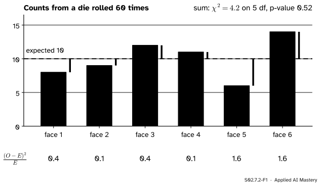
The simplest case is a die rolled 60 times (invented counts). A fair die expects 10 of each face.
S02.7.2-F1
Observed counts (blue) against the 10 a fair die expects. The purple gaps, squared and divided by 10, add to 4.2.
The gaps look uneven: face 5 came up only 6 times, face 6 came up 14. But a fair die rolled 60 times is never perfectly even. The question is whether 4.2 is a large total for a fair die, and the answer comes from the distribution of that total when the die really is fair.
Build it up
Step 1. Expected counts. The hypothesis gives each category a probability \(p_j\); with \(n\) observations, the expected count is \(E_j = n p_j\). For the fair die, \({60 \times \tfrac16} = 10\).
Step 2. Scaled squared gaps. A gap of 4 means more when 10 were expected than when 1,000 were. A count’s natural spread grows with its size (a count expected to be \(E\) has variance close to \(E\) when \(p_j\) is small), so each squared gap is divided by \(E_j\). Face 6 contributes \({(14 - 10)^2 / 10} = 1.6\).
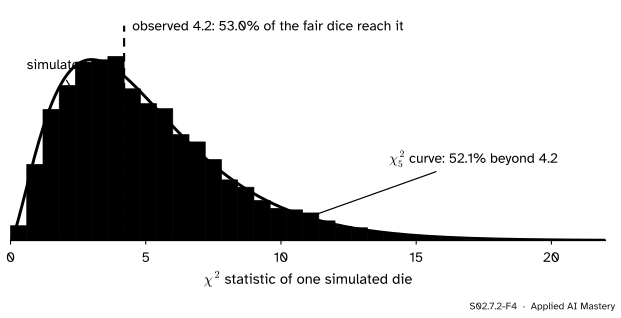
Step 3. Add, and ask how big chance makes it. The total 4.2 is the chi-square statistic. Roll a truly fair die 60 times, over and over, and compute it each time: its values pile up along the \(\chi^2_5\) curve of S02.1.4.
S02.7.2-F4
The statistic for 20,000 fair dice (seed 1). The \(\chi^2_5\) curve is an approximation, drawn in the model colour, and a good one here: 53.0 percent of the simulated dice reach 4.2 against 52.1 percent under the curve.
Step 4. Degrees of freedom. Six counts must add to 60, so once five are known the sixth is fixed: 5 free counts, 5 degrees of freedom. So the p-value is \({\Prob(\chi^2_5 \ge 4.2)} = 0.52\): this die gives no evidence of bias.
The formal statement
NoteDefinition: the chi-square statistic
For observed counts \(O_j\) and expected counts \(E_j\) over the categories,
\[
X^2 = \sum_j \frac{(O_j - E_j)^2}{E_j} .
\]
When \(H_0\) is true and every \(E_j\) is at least about 5, \(X^2\) approximately follows \(\chi^2_\nu\). The p-value is \({\Prob(\chi^2_\nu \ge X^2)}\): only large values count against \(H_0\).
The approximation is shown by simulation here, not proved. Its degrees of freedom are the number of counts that are free once everything used to compute the \(E_j\) has been fixed.
Goodness of fit.\(k\) categories with probabilities fixed by \(H_0\): \(\nu = k - 1\).
Independence in a two-way table. Rows \(g\) and columns \(j\) with counts \(O_{gj}\), row totals \(n_{g\cdot}\), column totals \(n_{\cdot j}\) and grand total \(n\). \(H_0\) says the row and column variables are independent, so
\[
\begin{aligned}
&\Prob(\text{row } g \text{ and column } j) \\
&\quad= \Prob(\text{row } g)\,\Prob(\text{column } j) .
\end{aligned}
\]
Estimate each factor by its margin, \({n_{g\cdot}/n}\) and \({n_{\cdot j}/n}\), and multiply by \(n\):
Degrees of freedom. With \(r\) rows and \(c\) columns, fix all the margins. Fill in the first \(r - 1\) rows and \(c - 1\) columns freely; the last entry of each row and of each column is then forced by its total. So \(\nu = (r - 1)(c - 1)\).
Small tables: Fisher’s exact test. When some \(E_{gj}\) are below 5, use the exact null distribution instead. For a 2 by 2 table with all margins fixed, one cell determines the rest, and under independence that cell follows the hypergeometric distribution of M06.2.4. Take 14 invented listings: in Centre 5 of 6 have a balcony, in South 2 of 8; 7 of the 14 have one. The chance of exactly 5 in Centre is
The two-sided p-value adds every table as unlikely or less (Centre count 0, 1, 5 or 6): \({352 / 3432} = 0.103\). The chi-square statistic for the same table is 4.67, p-value 0.031: with expected counts of only 3 and 4, the approximation claims a discovery the exact test does not.
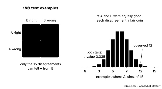
Paired counts: McNemar’s test. Classifier A gets 90 of 100 test examples right (the course’s running example) and classifier B, scored on the same examples, 81 (invented).
S02.7.2-F5
McNemar’s test. The 85 examples where the models agree say nothing about which is better. Under \(H_0\) each of the 15 disagreements goes either way with probability one half.
If the models are equally accurate, a disagreement is equally likely to favour either, so the number won by A is Binomial(15, 0.5). A won 12: the two-sided exact p-value is \({2 \times 576 / 32768} = 0.035\). The large-sample version is \({(12 - 3)^2 / (12 + 3)} = 5.4\) on 1 degree of freedom, p-value 0.020; Dietterich’s form subtracts 1 from \({\abs{12 - 3}}\) as a continuity correction, \({64/15} = 4.27\), p-value 0.039.
Worked example
Is a balcony independent of the district? The 120 invented listings of S01.5.4.
S02.7.2-F2
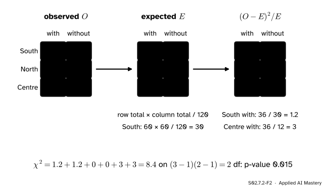
The test of independence, cell by cell: observed counts, the counts independence expects, and each cell’s contribution.
Margins. Rows: South 60, North 36, Centre 24. Columns: 60 with a balcony, 60 without.
Expected counts, \({E_{gj} = n_{g\cdot} n_{\cdot j}/n}\). South: \({60 \times 60 / 120} = 30\) in each column. North: 18 and 18. Centre: 12 and 12.
Contributions. South: \({(24 - 30)^2/30} = 1.2\) and \({(36 - 30)^2/30} = 1.2\). North: 0 and 0. Centre: \({(18 - 12)^2/12} = 3\) and \({(6 - 12)^2/12} = 3\).
Total \(X^2 = 8.4\) on \({(3 - 1)(2 - 1)} = 2\) degrees of freedom.
For 2 degrees of freedom the tail has a closed form, \({\Prob(\chi^2_2 \ge x)} = e^{-x/2}\), so the p-value is \(e^{-4.2} = 0.015\).
At level 0.05 the data reject independence: the share with a balcony does depend on the district. The contributions say where: Centre has 6 more balconies than independence predicts, South 6 fewer. Every expected count is at least 12, so the approximation is safe.
Code
From scratch: the statistic, the expected counts from the margins, and a simulation of the fair die.
Fisher’s and McNemar’s exact tests are sums of hypergeometric and binomial probabilities.
from math import combprobs = [comb(6, k) * comb(8, 7- k) for k inrange(7)] # Centre count k, out of comb(14, 7)fisher_p =sum(q for q in probs if q <= probs[5]) / comb(14, 7)mcnemar_p =2*sum(comb(15, k) for k inrange(4)) /2**15# A wins 12 of 15 disagreementsprint(probs, round(fisher_p, 3), round(mcnemar_p, 4))
[8, 168, 840, 1400, 840, 168, 8] 0.103 0.0352
The library versions. chi2_contingency applies Yates’s continuity correction whenever the table has 1 degree of freedom, so pass correction=False to get the statistic of the formula.
0.5209949534314052 8.4 2 0.014995576820477714
0.10256410256410256 4.666666666666666 0.030753561259274562 3.0 0.03515625
sklearn chi2 score for the balcony column: [4.2] [0.12245643]
sklearn.feature_selection.chi2 scores each feature column against the classes for screening. It treats the column’s values as counts, so a 0/1 balcony column scores only the “with” cells, \({1.2 + 0 + 3} = 4.2\), half of the full table’s 8.4. It is a ranking score for choosing features, not the test of independence.
Explore
This module’s interactive, the ANOVA decomposer, lives in lesson S02.7.3. For counts, the code above is the place to experiment: move one listing from Centre-with to Centre-without and watch the statistic fall.
Pitfalls
S02.7.2-F3
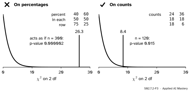
Wrong beside right. The same row shares, entered as percentages and as counts, give very different statistics.
“I’ll feed the table of percentages to the test; it shows the pattern better.”
The chi-square statistic grows in proportion to the number of observations: double every count and \(X^2\) doubles. Percentages pretend each row had 100 listings, 300 in all, and give \(X^2 = 26.3\) instead of 8.4. Always test the raw counts.
“The p-value is 0.031, so the 14 listings show a difference.”
With expected counts of 3 and 4 the chi-square curve is a poor guide to the statistic. Fisher’s exact test gives 0.103. When any expected count is below about 5, use an exact test.
“A chi-square test on the two classifiers’ right and wrong counts compares them.”
A table of 90 right and 10 wrong against 81 right and 19 wrong treats the 200 results as independent, but each test example appears twice. Use McNemar’s test on the disagreements. And a high sklearn.feature_selection.chi2 score ranks a feature; it is not a p-value to report.
Check yourself
Recall
1. Write the chi-square statistic and say what each part is.
Show answer
\(X^2 = {\sum_j (O_j - E_j)^2 / E_j}\): the observed counts \(O_j\), the counts \(E_j\) expected under \(H_0\), and a sum over all categories or cells.
2. How are expected counts found in a test of independence, and how many degrees of freedom does an \(r\) by \(c\) table have?
Show answer
\(E_{gj} = {n_{g\cdot} n_{\cdot j} / n}\), row total times column total over the grand total. The degrees of freedom are \((r - 1)(c - 1)\).
3. What are the chi-square statistic and p-value for the balcony table?
Show answer
\(X^2 = 8.4\) on 2 degrees of freedom, p-value \({e^{-4.2}} = 0.015\).
4. When should Fisher’s exact test replace the chi-square test?
Show answer
When expected counts are small, below about 5 in some cell, as in the 14-listing table (exact p-value 0.103 against 0.031 from the approximation).
5. Which counts does McNemar’s test use, and what is their null distribution?
Show answer
Only the examples on which the two classifiers disagree. Under \(H_0\) each goes either way with probability one half, so the count won by one model is Binomial(disagreements, 0.5).
Exercises
1.★ Another die is rolled 60 times and gives 5, 8, 9, 8, 10 and 20. Test whether it is fair.
Show solution
Expected 10 each. Squared gaps: 25, 4, 1, 4, 0, 100, sum 134; divided by 10, \(X^2 = 13.4\) on 5 degrees of freedom. stats.chi2.sf(13.4, 5) gives 0.020, below 0.05: face 6 alone contributes 10 of the 13.4.
2.★★ Design A got 30 clicks from 200 visitors and design B 50 from 200 (invented). Lay out the 2 by 2 table, find the expected counts and \(X^2\), and say what chi2_contingency returns by default.
Show solution
Rows A and B, columns clicked and not: 30, 170 and 50, 150. Margins: 200 per row, 80 clicked and 320 not. Expected: \({200 \times 80/400} = 40\) clicked and 160 not, in each row. Contributions: \({100/40} = 2.5\) twice and \({100/160} = 0.625\) twice, so \(X^2 = 6.25\) on 1 degree of freedom, p-value 0.012. By default chi2_contingency applies Yates’s correction for 1 degree of freedom and returns 5.64 with p-value 0.018; correction=False returns 6.25.
3.★★★ For two categories with \(H_0\) probability \(p\) for the first, show that the goodness-of-fit \(X^2\) equals \(z^2\), where \({z = (O_1 - np)/\sqrt{np(1 - p)}}\) is the z statistic for a proportion.
Show solution
\(O_2 = n - O_1\) and \(E_2 = n(1 - p)\), so \({O_2 - E_2} = -(O_1 - np)\). Then
Small or paired. Fisher’s exact test; McNemar’s binomial test on disagreements.
Sources and next steps
Sources. Each was opened and checked against this lesson on 15 November 2026.
MIT OpenCourseWare 18.05, Reading 19, Null Hypothesis Significance Testing III, Spring 2022 (free PDF). Section 4.5 defines Pearson’s statistic and the likelihood-ratio statistic \(G\); 4.5.1 counts degrees of freedom as the counts that can be set freely; 4.6 is the test for homogeneity.
David Diez, Mine Cetinkaya-Rundel and Christopher Barr, OpenIntro Statistics, fourth edition (free PDF). Section 6.3 tests goodness of fit; Section 6.4 is the chi-square test for two-way tables.
SciPy developers, chi2_contingency, chisquare and fisher_exact: expected counts from the margins, Yates’s correction when the degrees of freedom are 1, the guideline that counts be at least 5, and the hypergeometric null of the exact test.
scikit-learn developers, sklearn.feature_selection.chi2: chi-squared statistics between each non-negative feature and the class, for selecting features.