When no formula gives a statistic’s standard error, let the sample stand in for the population and resample it with replacement. Worked on the nine rents: the bootstrap standard error of the median and of the mean, and why a resample holds about 63 percent of the rows.
S02.8.1L2 Intermediate25 minIn review (what this means)
The maths and code on this page are checked by automated tests on every change, but an independent reader has not signed it off yet. Spot a mistake or a confusing step? Tell us.
State the plug-in principle and explain why the bootstrap resamples the sample with replacement and at its own size.
Compute a bootstrap standard error from scratch with numpy.random.default_rng and rng.integers, and read it off scipy.stats.bootstrap.
Derive the ideal bootstrap standard error of the mean and compare it with s divided by the square root of n.
Derive the chance (1 - 1/n)^n that a row is left out of a resample, and its limit 1/e.
The question
The nine flats of S01 have a median rent of 8 (hundreds of euros a month). How far would that median move if we could collect nine other flats? For the mean, \({s/\sqrt{n}}\) answers. For the median of nine skewed rents no simple formula does, and the same is true of most numbers a machine-learning model reports. Can the nine rents tell us their own uncertainty?
Intuition
The standard error of a statistic (S02.1.2) is the spread of its sampling distribution: compute the statistic on many samples from the population and see how much it varies. In the real world we have one sample and no population to draw more from.
The bootstrap makes the one sample play the part of the population. Draw nine rents from the nine, with replacement, compute the median, and do it again ten thousand times. The spread of those medians stands in for the spread we cannot see.
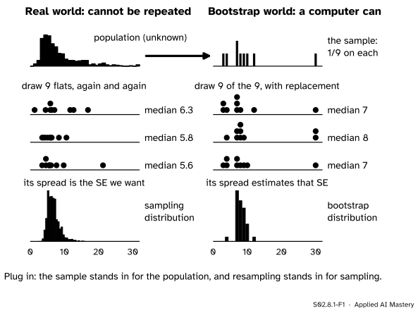
S02.8.1-F1
Two worlds. On the left, the sampling distribution we would like: medians of many samples from the population. On the right, what a computer can make: medians of many resamples from the one sample. The spread on the right estimates the spread on the left.
Read the two panels row by row. The population becomes the sample. Drawing a fresh sample becomes drawing a resample. The sampling distribution becomes the bootstrap distribution. Nothing new is learned about the population’s centre: the bootstrap only estimates how much a statistic wobbles from sample to sample.
Build it up
Step 1. Treat the sample as a population. Put the nine rents in a hat, one ball each: 7, 12, 3, 10, 30, 8, 9, 4, 7 for flats F1 to F9. Drawing one ball gives each rent probability 1/9. This little population is the empirical distribution of the sample, written \(\hat{F}_n\).
Step 2. Draw with replacement, n times. Draw a ball, write down its rent, put it back, and repeat until you have nine rents. Because each ball goes back, a flat can come out twice or not at all. The resample has the sample’s own size, because a standard error depends on \(n\): a resample of 90 would wobble far less than a sample of nine.
Step 3. Compute the statistic. The median of the resample is one replicate, written \(\cmodel{\hat\theta^*_1}\). The star marks anything computed in the bootstrap world.
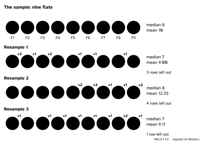
S02.8.1-F2
The first three resamples of the code below. Yellow rows were drawn, with a count of how often; dashed rows were left out. Each resample gives its own median and mean.
Step 4. Repeat K times. Ten thousand resamples give ten thousand replicates. Their histogram is the bootstrap distribution, and its standard deviation is the bootstrap standard error. The number of resamples \(\cparam{K}\) is ours to choose; the course writes \(K\) because \(B\) is a mini-batch.
The formal statement
NoteDefinition: the bootstrap standard error
Let \(x_1, \dots, x_n\) be a sample and \(\hat\theta\) a statistic computed from it. For \(k = 1, \dots, K\), draw a resample \(x^*_1, \dots, x^*_n\) by choosing \(n\) rows independently and uniformly from the \(n\) rows, and compute the replicate \(\hat\theta^*_k\). With \(\bar\theta^*\) the average of the replicates, the bootstrap standard error is
This is the plug-in principle: a quantity defined by the unknown population \(F\) is estimated by the same quantity computed with \(\hat{F}_n\) in place of \(F\). Here the quantity is the standard deviation of \(\hat\theta\) over samples of size \(n\). As \(K\) grows the estimate settles on the ideal bootstrap standard error, the exact standard deviation over all \({9^9}\) equally likely ordered resamples.
The mean, exactly. One draw \(X^*\) from \(\hat{F}_n\) takes each value \(x_i\) with probability \(1/n\), so its mean and variance are
The \(n\) draws are independent, so the variance of their mean is \({\operatorname{Var}^*(X^*)/n}\) (M06.7). And \(\hat\sigma^2\) divides by \(n\) where \(s^2\) divides by \({n - 1}\), so \({\hat\sigma^2 = s^2\,(n-1)/n}\). Together:
so the probability tends to \({e^{-1} = 0.368}\). Each row is in the resample with probability \({1 - (1 - 1/n)^n}\), so by adding these over the \(n\) rows the expected number of distinct rows is \({n\,(1 - (1-1/n)^n)}\): a share of 0.654 for \({n = 9}\) and of \({1 - 1/e = 0.632}\) for large \(n\), the birthday-problem warning of M06.2.2 in numbers.
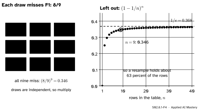
S02.8.1-F4
Left: why a given row is missed with probability \({(8/9)^9}\). Right: the same chance for any table size settles just under \(1/e\), so about 37 percent of the rows sit out each resample.
Go deeper: the exact bootstrap distribution of the median
For nine rows the ideal bootstrap distribution of the median can be listed without simulation. The median of a resample is at most \(v\) exactly when at least five of the nine draws are at most \(v\). Each draw is at most \(v\) with probability \(q\), the share of the rents at most \(v\), so
For \({v = 7}\), four of the nine rents (3, 4, 7, 7) are at most 7, so \({q = 4/9}\) and the sum is 0.3655. Taking differences between neighbouring values gives the probabilities 0.0014, 0.0289, 0.3351, 0.2690, 0.2207, 0.1145, 0.0289 and 0.0014 for the medians 3, 4, 7, 8, 9, 10, 12 and 30. Their standard deviation, the ideal bootstrap standard error of the median, is 1.630.
Worked example
One resample by hand. The code’s first resample draws rows 8, 6, 5, 3, 3, 1, 1, 1, 2. Their rents are 4, 8, 30, 3, 3, 7, 7, 7, 12. Sorted: 3, 3, 4, 7, 7, 7, 8, 12, 30. The fifth of nine is the median, \({\cmodel{\hat\theta^*_1} = 7}\). Rows F4, F7 and F9 were left out: three of nine, close to the expected \({9 \times 0.346 = 3.1}\).
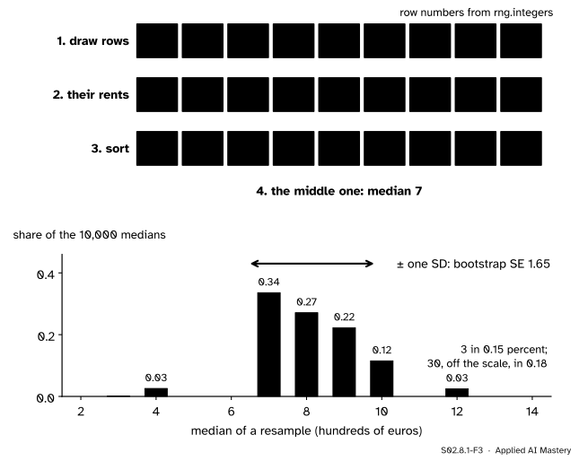
S02.8.1-F3
The worked example as a trace: one resample from row numbers to median, then the bar chart of all 10,000 medians and their standard deviation, the bootstrap standard error.
Ten thousand resamples. The medians land on only eight values, the eight different rents, because the median of nine rents is always one of the rents; the extremes 3 and 30 turn up in fewer than 2 resamples in 1,000. Their standard deviation is \({\widehat{\text{se}}_{\text{boot}} = 1.65}\), close to the ideal 1.63 of the deeper block.
The mean, for comparison. The rents have \({\bar{x} = 10}\) and squared deviations adding to 512, so \({s^2 = 512/8 = 64}\) and \({s = 8}\). The usual estimate is \({s/\sqrt{n} = 8/3 = 2.67}\). The ideal bootstrap value is
which is \({2.67 \times \sqrt{8/9}}\), and ten thousand resamples give 2.49. So the median of these rents is the steadier summary: its standard error, 1.65, is two thirds of the mean’s, because the penthouse at 30 moves the mean of every resample it lands in and almost never moves the median.
Code
From scratch: row numbers from rng.integers, then the statistic along each row.
import mathimport numpy as nprents = np.array([7, 12, 3, 10, 30, 8, 9, 4, 7], dtype=float) # F1 to F9, the nine flats of S01n, K =len(rents), 10_000rng = np.random.default_rng(0)rows = rng.integers(0, n, size=(K, n)) # K resamples, each n row numbers from 0 to n - 1resamples = rents[rows]medians = np.median(resamples, axis=1)means = resamples.mean(axis=1)se_median = medians.std(ddof=1)se_mean = means.std(ddof=1)s = rents.std(ddof=1)ideal_mean = math.sqrt(((rents - rents.mean()) **2).sum() / n / n)print("first resample:", rows[0] +1, "median", medians[0])print(f"bootstrap SE of the median {se_median:.2f}")print(f"bootstrap SE of the mean {se_mean:.2f}, ideal {ideal_mean:.2f}, s/sqrt(n) {s / math.sqrt(n):.2f}")left_out = np.mean([n -len(set(r)) for r in rows]) / nprint(f"share of rows left out per resample {left_out:.3f}; (1 - 1/n)^n = {(1-1/ n) ** n:.3f}")
first resample: [8 6 5 3 3 1 1 1 2] median 7.0
bootstrap SE of the median 1.65
bootstrap SE of the mean 2.49, ideal 2.51, s/sqrt(n) 2.67
share of rows left out per resample 0.345; (1 - 1/n)^n = 0.346
The exact distribution of the deeper block, with math.comb, confirms the simulation:
values = np.sort(np.unique(rents))cdf = [sum(math.comb(9, k) * q ** k * (1- q) ** (9- k) for k inrange(5, 10))for q in [np.mean(rents <= v) for v in values]]prob = np.diff([0.0] + cdf)centre = (prob * values).sum()ideal_median = math.sqrt((prob * (values - centre) **2).sum())print(dict(zip(values.tolist(), prob.round(4).tolist())))print(f"ideal bootstrap SE of the median {ideal_median:.3f}")
{3.0: 0.0014, 4.0: 0.0289, 7.0: 0.3351, 8.0: 0.269, 9.0: 0.2207, 10.0: 0.1145, 12.0: 0.0289, 30.0: 0.0014}
ideal bootstrap SE of the median 1.630
SciPy does the same resampling. scipy.stats.bootstrap takes a tuple of samples and a statistic, and its result carries the standard error beside the interval of the next lesson:
from scipy import statsresult = stats.bootstrap((rents,), np.median, n_resamples=9999, method="percentile", rng=np.random.default_rng(0))print(f"scipy bootstrap SE of the median {result.standard_error:.2f}")
scipy bootstrap SE of the median 1.65
Explore
S02.8-X1
Resampling machine
The nine rents are nine balls. Press Draw 1 to resample them and watch which balls light up and how often; the resample’s median drops onto the histogram. Draw a thousand and compare the standard error and the share of rows left out with 1.63 and 0.346. Switch to the mean, then to Shuffle mode, which belongs to lesson S02.8.3.
Pitfalls
S02.8.1-F5
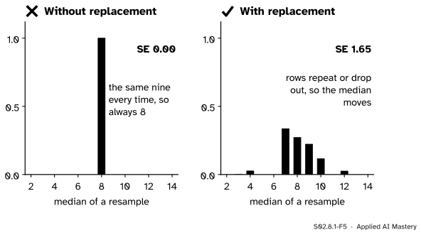
Wrong beside right. Drawing nine of nine without replacement only reorders the sample, so every “resample” has median 8 and the standard error comes out as zero.
“Resample the rows without replacement, so that no row counts twice.”
Nine rows drawn from nine without replacement are the same nine rows in a new order, and every statistic that ignores order comes out the same. The repeats and gaps are the point: they mimic how a fresh sample would contain different flats.
S02.8.1-F6
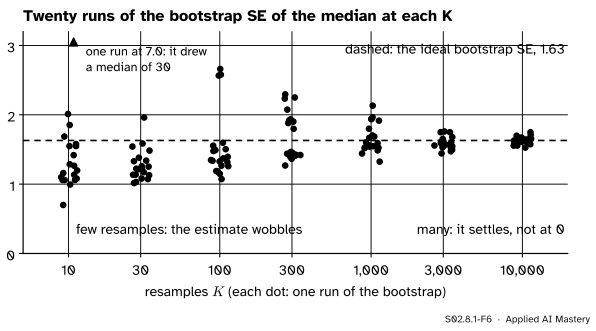
More resamples remove the noise of the simulation. With few, one rare replicate (a median of 30) can throw a run far off. They do not shrink the standard error, which settles at 1.63, the value fixed by the nine rents themselves.
“A million resamples will make the estimate more precise.”
The number of resamples \(\cparam{K}\) only controls Monte Carlo noise, the gap between a finite run and the ideal bootstrap. The standard error itself is fixed by the data; only more flats, a larger \(n\), make it smaller. A thousand resamples give a rough answer; Hesterberg recommends ten thousand for routine use, so that two people analysing the same data get the same interval.
“The bootstrap gives us more data.”
It gives no new information about the population: the replicates centre on the sample’s own statistic, not on the truth. If the nine flats are unusual, every resample inherits that. The bootstrap measures the wobble of an estimate, assuming the sample is a fair picture of the population, as a random sample (S01.2) is.
Check yourself
Recall
1. In the plug-in principle, what plays the part of the population?
Show answer
The empirical distribution of the sample, \(\hat{F}_n\): each of the \(n\) rows with probability \({1/n}\).
2. Why is the resample the same size as the sample?
Show answer
Because the spread of a statistic depends on the sample size. Resamples of another size would estimate the standard error for that size, not for ours.
3. What is the bootstrap standard error?
Show answer
The standard deviation of the \(K\) replicates \({\hat\theta^*_1, \dots, \hat\theta^*_K}\), with divisor \({K - 1}\).
4. What is the chance that a given row is left out of a resample of nine, and its limit for large \(n\)?
Show answer
\({(8/9)^9 = 0.346}\), tending to \({1/e = 0.368}\) as \(n\) grows.
5. For the mean, how does the ideal bootstrap standard error compare with \({s/\sqrt{n}}\)?
Show answer
It is smaller by the factor \({\sqrt{(n-1)/n}}\), because \(\hat{F}_n\) has variance \({\hat\sigma^2}\), with divisor \(n\), not \({s^2}\).
Exercises
1.★ A test set has 100 rows. Find the chance that row 1 is left out of one bootstrap resample, and the expected number of distinct rows in a resample.
Show solution
Each of the 100 draws misses row 1 with probability 0.99, so the chance is \({0.99^{100} = 0.366}\). Each row is in the resample with probability \({1 - 0.366 = 0.634}\), so the expected number of distinct rows is \({100 \times 0.634 = 63.4}\).
2.★★ For the sample 2, 4, 9, find the ideal bootstrap standard error of the mean and compare it with \({s/\sqrt{n}}\).
Show solution
The mean is \({\bar{x} = 5}\), and the squared deviations are 9, 1 and 16, adding to 26. So \({\hat\sigma^2 = 26/3}\) and the ideal bootstrap standard error is \({\sqrt{(26/3)/3} = \sqrt{26/9} = 1.700}\). With divisor \({n - 1}\), \({s^2 = 13}\) and \({s/\sqrt{3} = 2.082}\). The ratio is \({1.700/2.082 = 0.816 = \sqrt{2/3}}\), the factor \({\sqrt{(n-1)/n}}\).
3.★★★ For three distinct values \({a < b < c}\), find the exact bootstrap distribution of the median of a resample of three, and its standard deviation for 2, 4, 9.
Show solution
There are \({3^3 = 27}\) equally likely ordered resamples. The median is \(a\) when at least two of the three draws are \(a\): exactly two in \({3 \times 2 = 6}\) ways (choose the odd draw’s position and its value, \(b\) or \(c\)) and all three in 1 way, so \({\Prob = 7/27}\). By symmetry the median is \(c\) with probability \({7/27}\), which leaves \({13/27}\) for \(b\). For 2, 4, 9 the mean of the median is
so the variance is \({29.741 - 4.778^2} = 6.914\) and the ideal bootstrap standard error is 2.63.
Summary card
Resample the sample, with replacement, to see how much a statistic wobbles.
S02.8.1-F1
The sample stands in for the population.
Plug-in. Replace the population \(F\) by \(\hat{F}_n\), 1/n on each row.
Bootstrap SE. The standard deviation of \(K\) replicates \(\hat\theta^*_k\).
The mean. Ideal value \({\hat\sigma/\sqrt{n} = \sqrt{(n-1)/n}\; s/\sqrt{n}}\).
Left out. A row misses a resample with probability \({(1 - 1/n)^n \approx 0.368}\).
Sources and next steps
Sources. Each was opened and checked against this lesson on 15 November 2026.
Jeremy Orloff and Jonathan Bloom, Reading 24: Bootstrap confidence intervals, MIT OpenCourseWare 18.05, Spring 2022. Section 6.1 states the bootstrap principle (the empirical distribution stands in for the true one, and the variation of the resampled statistic for that of the statistic), section 6.2 explains why a resample has the sample’s size, and section 8 notes that resampling cannot improve the point estimate.
Tim Hesterberg, What Teachers Should Know about the Bootstrap, arXiv:1411.5279 (2014). Section 3.2 gives the narrowness factor \({\sqrt{(n-1)/n}}\) of the bootstrap standard error of the mean, section 3.3 notes that for odd \(n\) the bootstrap median is always one of the data values, and section 3.6 recommends ten thousand resamples for routine use.
SciPy, scipy.stats.bootstrap: the arguments n_resamples (default 9999), method and rng, and the result’s standard_error, the sample standard deviation of the bootstrap distribution.