When normality is doubtful, replace values by their ranks. The sign test, the Wilcoxon signed-rank test, the Mann-Whitney U test and the Kruskal-Wallis test, with exact null distributions counted by hand, and why U divided by its maximum is a classifier’s AUC.
S02.7.4L2 Intermediate25 minIn review (what this means)
The maths and code on this page are checked by automated tests on every change, but an independent reader has not signed it off yet. Spot a mistake or a confusing step? Tell us.
Run the sign test and the Wilcoxon signed-rank test on paired data, and find their exact p-values by counting sign patterns.
Compute the Mann-Whitney U statistic by counting pairs, relate it to the rank sum, and get its exact null distribution from all splits of the data.
Compute the Kruskal-Wallis statistic as an analysis of variance on ranks.
Explain why U divided by the number of pairs is the AUC of a classifier, and what a rank test does and does not compare.
The question
The ANOVA of the last lesson could not separate the districts, largely because of one penthouse. Move the penthouse from 30 to 60 and the evidence gets weaker. A test that only asks which flat rents for more than which would not care how far out the penthouse is. And a classifier’s AUC, the most common score for ranking models, turns out to be exactly such a test statistic.
From the last lesson
1. What do the between and within sums of squares of rent by district add up to, and what is \(F\)?
Show answer
\({234 + 278} = 512\), and \({F = 117/46.33} = 2.53\) on 2 and 6 degrees of freedom, p-value 0.160.
2. How is ANOVA’s \(F\) related to the pooled t statistic when there are two groups?
Show answer
\(F = t^2\), with the same p-value; for the two designs \(F = 3\) and \(t = \sqrt 3\).
Intuition
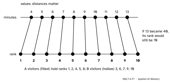
A rank is a value’s position when all the values are sorted: the smallest gets rank 1, the next rank 2, and so on. A rank test computes its statistic from the ranks alone. The ten minutes of the two page designs (invented) become the ranks 1 to 10.
S02.7.4-F1
From minutes to ranks. The order survives; the distances do not. Pushing the largest value further out cannot change any rank.
Ranks throw information away, the size of the gaps. In return the test no longer depends on the shape of the population, and pushing an extreme value further out changes nothing. Better still, under the null hypothesis every arrangement of the ranks is equally likely, so the exact null distribution can be found by counting.
Build it up
Step 1. The sign test (pairs). For the six analysts of S02.7.1, the differences old minus new were \(-1, 2, 3, 5, 6, 9\): five positive, one negative. If the new tool made no difference (the median difference is 0), each sign is a fair coin. Five or more of one sign out of six has probability \({2 \times (6 + 1)/64} = 0.219\). Using only signs wastes the sizes.
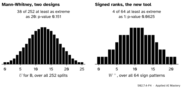
Step 2. Signed ranks (pairs). Rank the absolute differences, 1 to 6, and give each rank its difference’s sign. The negative ranks add to \(W^- = 1\) and the positive ranks to \(W^+ = 20\). Under \(H_0\) each of the \(2^6 = 64\) sign patterns is equally likely; only 2 of them give \(W^+ \le 1\), and 2 give \(W^+ \ge 20\), so the exact p-value is \({4/64} = 0.0625\).
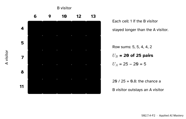
Step 3. Counting pairs (two groups). For the two designs, compare every A visitor with every B visitor: \(5 \times 5 = 25\) pairs. In 20 of them the B visitor stayed longer.
S02.7.4-F4
Exact null distributions, found by listing every case. Left: \(U\) for every way to choose which five of the ten times are B. Right: \(W^+\) for every pattern of six signs.
Step 4. Is 20 surprising? If the designs did not matter, any five of the ten times could have been B’s: \(\binom{10}{5} = 252\) splits, all equally likely. Counting \(U\) for each (F4, left), 19 splits give \(U \ge 20\) and 19 give \(U \le 5\), so the two-sided p-value is \({38/252} = 0.151\).
The formal statement
Ranks are taken over all the values together; tied values share the average of their ranks.
NoteDefinitions: three rank tests
Wilcoxon signed-rank (pairs): rank the nonzero \(\abs{d_i}\); \(W^+\) is the sum of the ranks of the positive \(d_i\) and \(W^-\) of the negative ones. scipy reports the smaller of the two.
Mann-Whitney U (two groups): \(U_B\) is the number of pairs \((a, b)\) with \(b > a\), a tie counting one half. Likewise \(U_A\), and \({U_A + U_B} = n_A n_B\).
Kruskal-Wallis H (\(k\) groups): the one-way ANOVA of S02.7.3 on the ranks \(r\), \({H = (N - 1)\,SS_B / SS_T}\), approximately \(\chi^2_{k-1}\) under \(H_0\) when the groups are not too small.
U from the rank sum. Sort the B values and let the \(j\)-th smallest have overall rank \(r_{(j)}\). Below it sit \({r_{(j)} - 1}\) values, of which \({j - 1}\) are B’s; the rest, \({r_{(j)} - j}\), are A’s it beats. Adding over \(j\):
where \(R_B\) is the sum of B’s ranks. For the designs, \({R_B = 3 + 6 + 7 + 9 + 10} = 35\) and \({U_B = 35 - 15} = 20\).
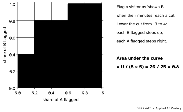
U is the AUC. Treat the minutes as a score that flags “shown design B”. As the cut falls, the ROC curve of ML01.7.3 steps up for each B flagged and right for each A flagged. Each step right, at an A value, runs at a height equal to the share of B values above that A value. So the area, a sum of columns of width \({1/n_A}\), counts the pairs in which B outscores A:
The minutes as a classifier’s score for “shown B”. The staircase encloses 20 of the 25 cells of the unit square: the AUC is the Mann-Whitney \(U\) divided by the number of pairs.
So \(U/(n_A n_B)\) estimates \({\Prob(B > A)}\), the chance that a random B outscores a random A, and the Mann-Whitney test asks whether that chance is \(\tfrac12\). A model’s AUC of 0.8 is the same number as a rank test’s effect size.
Kruskal-Wallis on the flats. Rents 3, 4, 7, 7, 8, 9, 10, 12, 30 get ranks 1, 2, 3.5, 3.5, 5, 6, 7, 8, 9. Rank sums: South 8, North 14, Centre 23; mean ranks 2.67, 4.67 and 7.67 around the grand mean rank 5. Then
where 60 is \({N(N^2 - 1)/12}\) for nine untied ranks and the tie at 7 removes 0.5. So \({H = 8 \times 38 / 59.5} = 5.11\) and the p-value from \(\chi^2_2\) is \({e^{-5.11/2}} = 0.078\), against 0.160 for the ANOVA. The penthouse has rank 9 whether it rents for 13 or 1,300.
Worked example
Did design B hold visitors longer? A: 4, 5, 7, 8, 11. B: 6, 9, 10, 12, 13.
S02.7.4-F2
Every A visitor against every B visitor. The green cells, where B stayed longer, number \(U_B = 20\).
Count, row by row, the B values above each A value: 5, 5, 4, 4, 2. So \(U_B = 20\) and \({U_A = 25 - 20} = 5\).
Check with ranks: B holds ranks 3, 6, 7, 9, 10, so \({R_B = 35}\) and \({35 - 15} = 20\).
Null distribution: all 252 splits (F4). 19 give \(U_B \ge 20\); by symmetry 19 give \(U_B \le 5\).
Two-sided p-value \({38/252} = 0.151\). Not significant at 0.05, like the t-test’s 0.122.
Effect size: \({20/25} = 0.8\), an estimate that a B visitor outstays an A visitor four times in five.
Code
From scratch: counts, ranks and full enumeration of the null distributions.
import itertoolsimport numpy as npfrom scipy import statsA = np.array([4, 5, 7, 8, 11.]); B = np.array([6, 9, 10, 12, 13.]) # the two designs (invented)d = np.array([20, 25, 31, 38, 44, 52.]) - np.array([21, 23, 28, 33, 38, 43.]) # the tool, old minus newdef u_stat(b, a):returnsum((x > y) +0.5* (x == y) for x in b for y in a)pooled = np.concatenate([A, B])u_null = [u_stat(pooled[list(s)], np.delete(pooled, list(s))) for s in itertools.combinations(range(10), 5)]u_obs = u_stat(B, A)p_u = np.mean([u >= u_obs or u <=25- u_obs for u in u_null])ranks = stats.rankdata(np.abs(d))w_plus = ranks[d >0].sum()w_null = [sum(r for r, s inzip(range(1, 7), signs) if s) for signs in itertools.product([0, 1], repeat=6)]p_w = np.mean([w <=21- w_plus or w >= w_plus for w in w_null])p_sign =2*sum(stats.binom.pmf(k, 6, 0.5) for k in (5, 6))print("U =", u_obs, " p =", round(p_u, 3), "| W+ =", w_plus, " p =", p_w, "| sign test p =", round(p_sign, 3))rents = np.array([3, 8, 4, 7, 10, 7, 12, 30, 9.])group = np.repeat([0, 1, 2], 3)r = stats.rankdata(rents)ss_b =sum(3* (r[group == g].mean() - r.mean()) **2for g inrange(3))ss_t = ((r - r.mean()) **2).sum()h = (len(r) -1) * ss_b / ss_tprint("ranks:", r, " H =", round(h, 3), " p =", round(np.exp(-h /2), 3))
U = 20.0  p = 0.151 | W+ = 20.0  p = 0.0625 | sign test p = 0.219
ranks: [1.  5.  2.  3.5 7.  3.5 8.  9.  6. ]  H = 5.109  p = 0.078
The library calls, and the AUC from scikit-learn.
from sklearn.metrics import roc_auc_scoreprint(stats.wilcoxon(d))print(stats.mannwhitneyu(B, A, method="exact"))print(stats.kruskal([3, 8, 4], [7, 10, 7], [12, 30, 9]))print(stats.kruskal([3, 8, 4], [7, 10, 7], [12, 60, 9]).statistic, "with the penthouse at 60")auc = roc_auc_score([0] *5+ [1] *5, np.concatenate([A, B]))print("AUC:", auc)
WilcoxonResult(statistic=np.float64(1.0), pvalue=np.float64(0.0625))
MannwhitneyuResult(statistic=np.float64(20.0), pvalue=np.float64(0.15079365079365079))
KruskalResult(statistic=np.float64(5.109243697478988), pvalue=np.float64(0.07772161703842191))
5.109243697478988 with the penthouse at 60
AUC: 0.8
mannwhitneyu returns the U of its first argument. Its default method="auto" is exact when one group has at most 8 values and there are no ties; wilcoxon is exact for up to 50 differences without ties or zeros.
Explore
This module’s interactive, the ANOVA decomposer, lives in lesson S02.7.3. Its read-out gives \(F\) and the Kruskal-Wallis \(H\) of this lesson side by side: drag the penthouse and watch \(F\) move while \(H\) holds still. Its Ranks button shows the ranks that \(H\) is computed from.
Pitfalls
S02.7.4-F3
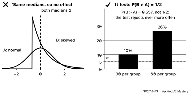
Wrong beside right. Two populations with the same median, where a random B still beats a random A 55.7 percent of the time. Rejection rates from 2,000 simulated pairs of samples per size (seed 4).
“The Mann-Whitney test compares medians.”
It compares \({\Prob(B > A)}\) with one half. Two populations can share a median and still differ on that score, as in the figure, and then the test rejects more and more often as the samples grow. It is a test of medians only if the two populations have the same shape, one shifted from the other.
“Rank tests make no assumptions.”
They drop normality, not independence. The signed-rank test also assumes the differences are symmetric about their median under \(H_0\), and the Kruskal-Wallis p-value uses a chi-square approximation that scipy recommends only for groups of at least 5. For the flats the exact permutation p-value, counted over all 1,680 ways to deal nine ranks into three groups of three, is \({132/1680} = 0.079\), close to 0.078 here, but that has to be checked, not assumed.
“For paired data, Mann-Whitney is the rank version of the t-test.”
Paired data need the paired rank test, the signed-rank test, for the same reason as in S02.7.1. Mann-Whitney on the tool’s old and new times would compare analysts with each other.
Check yourself
Recall
1. What are \(W^+\) and \(W^-\) for the tool, and the exact p-value of the signed-rank test?
Show answer
\(W^+ = 20\) and \(W^- = 1\) (the only negative difference has the smallest rank). The p-value is \({4/64} = 0.0625\).
2. How is the Mann-Whitney \(U_B\) defined, and what is it for the two designs?
Show answer
The number of (A, B) pairs in which B is larger, ties counting a half. For the designs \(U_B = 20\) of 25.
3. How is \(U_B\) related to the rank sum \(R_B\)?
Show answer
\(U_B = R_B - {n_B(n_B + 1)/2}\); for the designs \({35 - 15} = 20\).
4. Why is \({U_B/(n_A n_B)}\) the AUC?
Show answer
Both count the share of (A, B) pairs that the score orders correctly: the area under the ROC staircase is made of one cell for each such pair. Here \({20/25} = 0.8\).
5. What is the Kruskal-Wallis \(H\) for rent by district, and why does the penthouse not affect it?
Show answer
\(H = 5.11\), p-value 0.078. \(H\) uses ranks, and the penthouse keeps rank 9 however high its rent.
Exercises
1.★ Seven paired differences are 3, −2, 5, 6, 4, 8, 7. Find the sign test’s and the signed-rank test’s exact two-sided p-values.
Show solution
Sign test: 6 positive of 7, so \({2 \times (7 + 1)/128} = 0.125\). Signed ranks: the absolute values 2, 3, 4, 5, 6, 7, 8 get ranks 1 to 7, and only the −2 is negative, so \(W^- = 1\). Among the \(2^7 = 128\) sign patterns, 2 give \(W^- \le 1\) and 2 give \(W^+ \le 1\), so the p-value is \({4/128} = 0.031\). The ranks use the fact that the one negative difference is the smallest.
2.★★ A classifier scores three positive examples 0.9, 0.8 and 0.4 and four negative examples 0.7, 0.3, 0.2 and 0.1. Compute \(U\) for the positives and the AUC.
Show solution
0.9 beats all 4 negatives, 0.8 beats all 4, and 0.4 beats 0.3, 0.2 and 0.1, so \(U = 11\) of \({3 \times 4} = 12\) pairs, and the AUC is \({11/12} = 0.917\). roc_auc_score([1, 1, 1, 0, 0, 0, 0], [0.9, 0.8, 0.4, 0.7, 0.3, 0.2, 0.1]) gives the same.
3.★★★ With no ties, the ranks are \(1, \dots, N\). Show that \({SS_T = N(N^2 - 1)/12}\), and deduce the usual formula \({H = \frac{12}{N(N + 1)}\sum_g R_g^2/n_g - 3(N + 1)}\), where \(R_g\) is group \(g\)’s rank sum.
Show solution
The mean rank is \({(N + 1)/2}\). Using \({\sum r^2 = N(N + 1)(2N + 1)/6}\),
For the flats this gives \({\tfrac{12}{90} \times 263} - 30 = 5.07\); the tie at 7 makes \(SS_T\) 59.5 instead of 60, which is why scipy’s tie-corrected value is 5.11.
Summary card
Rank the values, then count: the order counts, the distances do not.
AUC.\({U/(n_A n_B)} = 0.8\), an estimate of \({\Prob(B > A)}\).
Kruskal-Wallis. ANOVA on ranks: \(H = 5.11\), p-value 0.078.
Sources and next steps
Sources. Each was opened and checked against this lesson on 15 November 2026.
SciPy developers, scipy.stats.wilcoxon, scipy.stats.mannwhitneyu and scipy.stats.kruskal. The two-sided signed-rank statistic is the smaller rank sum, exact for up to 50 differences without ties or zeros; mannwhitneyu returns U for its first sample, with \({U_2 = n_1 n_2 - U_1}\), and is exact under "auto" when one sample has at most 8 values and there are no ties; kruskal corrects H for ties, uses the chi-square approximation and advises at least 5 values per group.
Tom Fawcett, An introduction to ROC analysis, Pattern Recognition Letters 27, 861 to 874, 2006. Section 7: the AUC equals the probability that the classifier ranks a randomly chosen positive above a randomly chosen negative, which is equivalent to the Wilcoxon test of ranks.
Next. S02.8 builds null distributions by shuffling instead of formulas: the permutation test of S02.8.3 gives the same 38 of 252 for the two designs’ difference in means.