Every t-test divides a difference by its standard error and reads the result against a t curve. Run the one-sample, paired and two-sample tests by hand, see why pairing removes the spread between subjects, and know when to use Welch’s version.
S02.7.1L2 Intermediate25 minIn review (what this means)
The maths and code on this page are checked by automated tests on every change, but an independent reader has not signed it off yet. Spot a mistake or a confusing step? Tell us.
Compute a t statistic as an estimate’s distance from its null value in standard errors, and read its p-value from the t distribution with the right degrees of freedom.
Run the one-sample, paired, pooled two-sample and Welch t-tests by hand and with scipy.stats.
Explain with the variance of a difference why a paired design removes the spread between subjects.
Recognise that comparing two models on the same test examples is a paired problem.
The question
Six analysts timed themselves on one task with their old tool and then with a new one. Five of the six were faster with the new tool, by 4 minutes on average. Is the new tool really faster, or could a gap like that turn up by chance? The answer depends on one fact that is easy to forget: the same six people used both tools. Machine learning meets the same question every time two models are scored on the same test set.
Intuition
A t-test asks whether a difference is large compared with the noise it was measured through. It divides the difference by its standard error, the yardstick of S02.1.2, and calls the ratio \(t\). A \(t\) near 0 is what chance alone produces; a \(t\) far from 0 is hard to explain by chance.
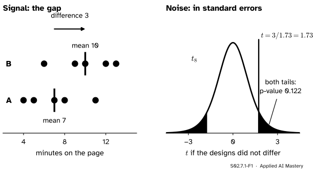
Take the two page designs of the course (invented): five visitors shown design A stayed 4, 5, 7, 8 and 11 minutes, five shown design B stayed 6, 9, 10, 12 and 13.
S02.7.1-F1
The two designs. The means differ by 3 minutes; the standard error of that difference is 1.73, so \(t = 1.73\). If the designs did not differ, a \(t\) at least that far from 0 would turn up 12.2 percent of the time.
The gap of 3 minutes is only 1.73 standard errors. The t curve on the right says how often chance alone would give a gap at least that large, in either direction: 12.2 percent of the time. That is the p-value of S02.5, and here it is too large to rule chance out.
Everything in this lesson is that picture with a different signal and a different yardstick.
Build it up
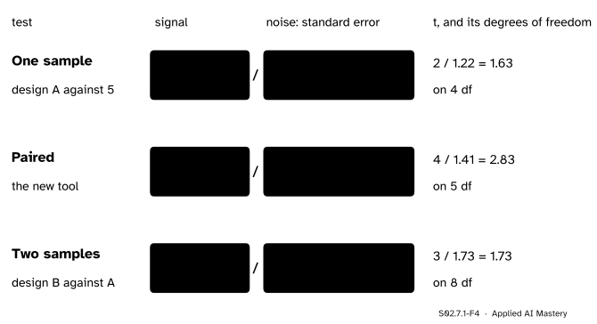
Step 1. One sample against a fixed value. Suppose the old page held visitors for 5 minutes on average (invented). Is design A’s mean of 7 different? The signal is \({\bar x - \mu_0} = 2\). The noise is the estimated standard error \({s / \sqrt{n}}\) with \(s^2 = 7.5\) and \(n = 5\): \({\sqrt{7.5} / \sqrt{5}} = 1.225\). So \(t = 1.63\). For a normal population this ratio follows \(t_{n-1}\), the result of S02.1.4, so the p-value comes from \(t_4\): 0.178. The 95 percent interval of S02.4.2, 3.60 to 10.40, contains 5, which is the same verdict (S02.5.4).
Step 2. Pairs become one sample. The six analysts give six differences, old minus new: \(-1, 2, 3, 5, 6, 9\). Once each analyst is reduced to one number, the question “is the new tool faster?” is the one-sample question “is the mean difference 0?”. Step 1 applies unchanged.
Step 3. Two independent groups. Design A and design B were seen by different visitors, so there are no pairs to subtract. The signal is \({\bar x_B - \bar x_A}\), and its standard error must include the noise of both means.
S02.7.1-F4
One recipe, three tests. Each \(t\) is a signal (vermillion) divided by its estimated standard error (purple), read against a t curve whose degrees of freedom come from the sample sizes.
The formal statement
NoteDefinition: the t statistic
For an estimate \(\hat\theta\) of \(\theta\), a null value \(\theta_0\) and an estimated standard error \(\widehat{\mathrm{se}}\), the t statistic is
\[
T = \frac{\hat\theta - \theta_0}{\widehat{\mathrm{se}}} .
\]
For normal data and \(H_0\) true, \(T\) follows \(t_\nu\) exactly in the one-sample, paired and pooled cases below, and approximately in Welch’s. The two-sided p-value is \({\Prob(\abs{T_\nu} \ge \abs{t})}\).
One sample.\(T = {(\bar x - \mu_0) / (s / \sqrt{n})}\) with \(\nu = n - 1\) (S02.1.4).
Paired. With pairs \((x_i, y_i)\) write \(d_i = x_i - y_i\). Then \(T = {\bar d / (s_d / \sqrt{n})}\) with \(\nu = n - 1\): the one-sample test on the \(d_i\) with \(\mu_0 = 0\).
When the two measurements share a source of spread (the same analyst, the same test example), the covariance is large and positive, and the subtraction removes it. For the tool data the sample variances are 144 (old) and 74 (new) and the sample covariance is 103, so
\[
144 + 74 - 2 \times 103 = 12 ,
\]
which is exactly \(s_d^2\), the variance of the six differences. Analysts differ from each other by a lot; each analyst’s two times differ by little.
Two independent samples, pooled. For independent groups the covariance term is 0. If both groups have the same standard deviation \(\sigma\), then \(\operatorname{Var}(\bar X_A) = {\sigma^2 / n_A}\) and \(\operatorname{Var}(\bar X_B) = {\sigma^2 / n_B}\), so
The ratio is then only approximately \(t\); Welch’s approximation gives the degrees of freedom (stated, not derived), with \(a = {s_A^2 / n_A}\) and \(b = {s_B^2 / n_B}\):
For the designs, \(a = b = 1.5\), so \({\nu = 9 / (2.25/4 + 2.25/4)} = 8\): the two versions agree exactly here because the sizes and variances are equal. They do not always agree.
S02.7.1-F5
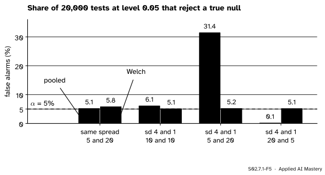
Simulated false alarms when the two means are equal (seed 7, 20,000 pairs of normal samples per setting). When the smaller group is the noisier one, the pooled test rejects a true null 31 percent of the time instead of 5; Welch’s stays near 5 in every setting.
Pooling averages the two variances with weights set by the sample sizes. When the large group is the quiet one, the pooled \(s^2\) is too small for the noisy small group, the standard error is too small and \(t\) too large. Welch’s test costs almost nothing when the variances are equal, so it is a safe default.
Worked example
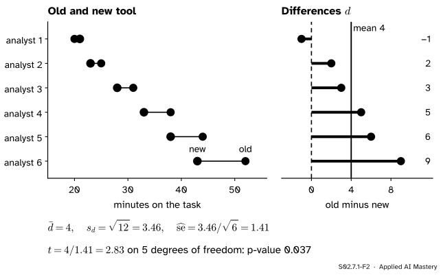
Is the new tool faster? Old and new times for the six analysts are 20, 25, 31, 38, 44, 52 and 21, 23, 28, 33, 38, 43 minutes (invented).
S02.7.1-F2
The paired test, step by step: subtract within each analyst, then run a one-sample test on the six differences.
Differences, old minus new: \(-1, 2, 3, 5, 6, 9\). Their sum is 24, so \(\bar d = 4\).
Deviations from 4: \(-5, -2, -1, 1, 2, 5\). Squares: 25, 4, 1, 1, 4, 25, sum 60. So \({s_d^2 = 60 / 5} = 12\) and \(s_d = 3.46\).
Standard error: \({3.46 / \sqrt{6}} = 1.41\).
\(t = {4 / 1.41} = 2.83\) on \(\nu = 5\) degrees of freedom.
Two-sided p-value: \({\Prob(\abs{T_5} \ge 2.83)} = 0.037\). At level 0.05 the data reject “no change”. A 95 percent interval for the mean saving is \({4 \pm 2.571 \times 1.41}\), 0.36 to 7.64 minutes.
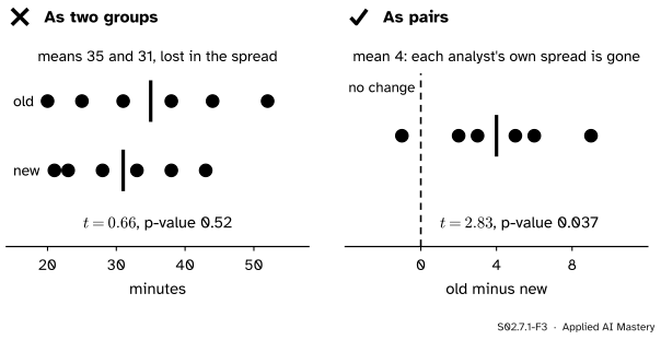
The same data, analysed wrongly. Treat the old and new times as two unrelated groups of six. The means are 35 and 31, still 4 apart. But now the noise is the spread between analysts: \(s^2 = 144\) and \(74\), so \({s_{\text{pool}}^2 = (144 + 74)/2} = 109\) and
Then \(t = {4 / 6.03} = 0.66\) on 10 degrees of freedom, p-value 0.52. The same 4 minutes look like nothing, because the yardstick now includes how much faster some analysts are than others.
Code
From scratch: the three statistics, with the t curve’s tail from scipy.stats.t.sf.
import numpy as npfrom scipy import statsA = np.array([4, 5, 7, 8, 11.]); B = np.array([6, 9, 10, 12, 13.]) # the two designs (invented)old = np.array([20, 25, 31, 38, 44, 52.]); new = np.array([21, 23, 28, 33, 38, 43.]) # the tool (invented)def t_one(x, mu0): t = (x.mean() - mu0) / (x.std(ddof=1) / np.sqrt(len(x)))return t, len(x) -1def t_pooled(a, b): na, nb =len(a), len(b) s2 = ((na -1) * a.var(ddof=1) + (nb -1) * b.var(ddof=1)) / (na + nb -2)return (b.mean() - a.mean()) / np.sqrt(s2 * (1/ na +1/ nb)), na + nb -2def p_two_sided(t, df):return2* stats.t.sf(abs(t), df)d = old - newfor name, (t, df) in [("A against 5", t_one(A, 5)), ("paired tool", t_one(d, 0)), ("B against A", t_pooled(A, B)), ("tool as two groups", t_pooled(new, old))]:print(f"{name:20s} t = {t:.3f} df = {df} p-value = {p_two_sided(t, df):.3f}")print("covariance of old and new:", np.cov(old, new)[0, 1], " variance of d:", d.var(ddof=1))
A against 5          t = 1.633  df = 4  p-value = 0.178
paired tool          t = 2.828  df = 5  p-value = 0.037
B against A          t = 1.732  df = 8  p-value = 0.122
tool as two groups   t = 0.664  df = 10  p-value = 0.522
covariance of old and new: 103.0  variance of d: 12.0
A check by simulation: if the true mean difference were 0, how often would six normal differences give \(\abs{t} \ge 2.83\)? The t curve says 3.7 percent.
The library calls. ttest_rel is the paired test; ttest_ind is pooled by default and Welch’s with equal_var=False; each result has a confidence_interval() method.
one = stats.ttest_1samp(A, 5)paired = stats.ttest_rel(old, new)welch = stats.ttest_ind(B, A, equal_var=False)print(one.statistic, one.pvalue)print(paired.statistic, paired.pvalue, paired.confidence_interval())print(welch.statistic, welch.pvalue, welch.df, welch.confidence_interval())
This module’s interactive, the ANOVA decomposer, lives in lesson S02.7.3. It compares three groups at once; with only two groups, the F statistic it shows would be exactly the square of the pooled \(t\) of this lesson.
Pitfalls
S02.7.1-F3
Wrong beside right. The same twelve times, compared as two groups (left) and as six pairs (right).
“Old and new are two samples, so I run a two-sample test.”
Two columns are not always two samples. When each row is one subject measured twice, the rows are pairs, and only the paired test removes the spread between subjects. Here it is the difference between p-value 0.52 and p-value 0.037.
“Model B beat model A by 1.5 points of accuracy on the test set; a two-sample test on the two accuracies tells me if that is real.”
Both models were scored on the same test examples, so their results are paired: many examples are easy for both and some are hard for both. Compare them example by example, with a paired t-test on per-example losses or McNemar’s test on right and wrong (S02.7.2). An unpaired test throws that pairing away and loses power.
“The groups have different sizes, but the pooled test is the textbook one.”
When the smaller group is the noisier one, pooling understates the standard error and the false alarm rate can reach 31 percent at a nominal 5 (F5). Use Welch’s test (equal_var=False) unless you have a reason to believe the variances are equal.
Check yourself
Recall
1. What does every t statistic divide by what?
Show answer
An estimate’s distance from its null value, \({\hat\theta - \theta_0}\), by the estimated standard error of the estimate.
2. How is a paired t-test turned into a one-sample test?
Show answer
Subtract within each pair, \(d_i = x_i - y_i\), and test whether the mean of the \(d_i\) is 0 with \(T = {\bar d / (s_d / \sqrt{n})}\) on \(n - 1\) degrees of freedom.
3. Give the paired \(t\) and p-value for the tool data, and the values when the same data are analysed as two independent groups.
Show answer
Paired: \(t = 2.83\) on 5 degrees of freedom, p-value 0.037. As two groups: \(t = 0.66\) on 10, p-value 0.52.
A large positive covariance between the two measurements of one subject is subtracted away. For the tool, \(144 + 74 - 206 = 12\).
5. How do the pooled and Welch two-sample tests differ?
Show answer
The pooled test assumes one shared variance and estimates it by \(s_{\text{pool}}^2\), with \(n_A + n_B - 2\) degrees of freedom. Welch’s uses \({\sqrt{s_A^2/n_A + s_B^2/n_B}}\) as the standard error and approximate degrees of freedom; it stays reliable when the variances differ.
Exercises
1.★ Test whether design B’s mean time differs from 7 minutes. Give \(t\), the degrees of freedom and the p-value (from code or a table).
Show solution
\(\bar x = 10\), \(s^2 = 7.5\), \(n = 5\), so \({\widehat{\mathrm{se}} = \sqrt{7.5/5}} = 1.225\) and \({t = 3 / 1.225} = 2.45\) on 4 degrees of freedom. 2 * stats.t.sf(2.449, 4) gives a p-value of 0.070: not significant at 0.05, though closer than design A against 5.
2.★★ Two models are scored on the same eight test batches. Model A’s log loss minus model B’s is 0.03, 0.05, −0.01, 0.04, 0.02, 0.06, 0.01, 0.04. Is B better? Which test, and what does it give?
Show solution
The batches are shared, so the test is paired: a one-sample t-test on the eight differences. \(\bar d = {0.24 / 8} = 0.03\); the deviations from 0.03 are 0, 0.02, −0.04, 0.01, −0.01, 0.03, −0.02, 0.01, whose squares add to 0.0036, so \({s_d^2 = 0.0036 / 7}\) and \(s_d = 0.0227\). Then \({\widehat{\mathrm{se}} = 0.0227 / \sqrt{8}} = 0.0080\) and \(t = 3.74\) on 7 degrees of freedom, p-value 0.0072. B’s loss is lower on average, and chance alone would rarely give a gap this steady. stats.ttest_rel(loss_a, loss_b) gives the same.
3.★★★ Show that when \(n_A = n_B = n\), the pooled and Welch t statistics are equal for any data. Do their degrees of freedom have to be equal too?
Show solution
With equal sizes, \({s_{\text{pool}}^2 = (s_A^2 + s_B^2)/2}\), so the pooled squared standard error is
which is Welch’s. The numerators are the same, so the statistics are equal. The degrees of freedom need not be: Welch’s \(\nu\) equals \(2n - 2\) only when \(s_A^2 = s_B^2\) (then \(a = b\) and \({\nu = 4a^2 / (2a^2/(n-1))} = 2(n - 1)\)), and is smaller otherwise, so the p-values differ. For the tool data analysed as groups, Welch’s \(\nu\) is 9.07 instead of 10.
Summary card
A t statistic is a difference measured in standard errors.
S02.7.1-F1
Signal over noise, read on \(t_\nu\).
One sample.\({(\bar x - \mu_0)/(s/\sqrt{n})}\) on \(n - 1\) df.
Paired. The one-sample test on the differences \(d_i\).
Two samples.\({(\bar x_B - \bar x_A)/\widehat{\mathrm{se}}}\), pooled or Welch.
Pairing. Removes \({2\operatorname{Cov}(X, Y)}\) from the noise.
Sources and next steps
Sources. Each was opened and checked against this lesson on 15 November 2026.
MIT OpenCourseWare 18.05, Reading 19, Null Hypothesis Significance Testing III, Spring 2022 (free PDF). Section 4.2 gives the one-sample t-test; 4.3.1 the two-sample test with pooled variance and \(n + m - 2\) degrees of freedom; 4.3.2 Welch’s test with its degrees-of-freedom formula; 4.3.3 the paired test, noted as “just a one-sample t-test” on the differences.
David Diez, Mine Cetinkaya-Rundel and Christopher Barr, OpenIntro Statistics, fourth edition (free PDF). Section 7.1 covers the t-distribution and one mean, 7.2 paired data, and 7.3 the difference of two means.