Find the power of any test on any population by simulation, then see what low power does to the results that do reach significance: they exaggerate the effect and can get its sign wrong, the winner’s curse of leaderboards. And why power computed after the fact tells nothing new.
S02.6.4L2 Intermediate25 minIn review (what this means)
The maths and code on this page are checked by automated tests on every change, but an independent reader has not signed it off yet. Spot a mistake or a confusing step? Tell us.
Estimate the power of any test by simulation, give its Monte Carlo standard error, and run scipy.stats.power.
Define Type S and Type M errors and show by simulation that significant results from a low-power study exaggerate the effect.
Explain the winner’s curse of a leaderboard as the same selection effect.
Show that observed power is a function of the p-value and so adds nothing to it.
The question
A team shows each of two page designs to five visitors. Design B wins by four minutes, p-value 0.03: significant. Should the team believe four minutes? Suppose the real gain is one minute. Then a study this small reaches significance only about one time in twelve, and when it does, the estimate it reports averages almost four minutes. The same arithmetic makes the top model on a leaderboard look better than it is.
From the last lesson
1. How many standard errors must an effect span for 80 percent power at level 0.05 two-sided?
Show answer
2.80: 1.96 from the null to the cut-off, plus 0.84 from the cut-off to the alternative’s centre.
2. The effect to detect halves. What happens to the sample size?
Show answer
It is multiplied by four, because \(n\) grows like \({1/\delta^2}\).
Intuition
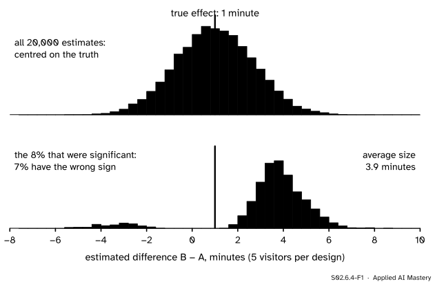
Imagine the designs study run 20,000 times when the true gain is one minute, and look at every estimate it would produce, then at the ones that reached significance.
S02.6.4-F1
The significance filter. The estimates are centred on the true one minute, but a study this small can only be significant when it is lucky by a lot, so the significant estimates sit far from the truth: too large, or on the wrong side of zero.
The top histogram is honest: the estimates scatter widely, but around the truth. The bottom one is what gets reported if only significant results count. To be significant with five visitors per design, an estimate has to be several minutes from zero, so every surviving estimate is several times the true effect. A few survive on the wrong side, pointing the wrong way.
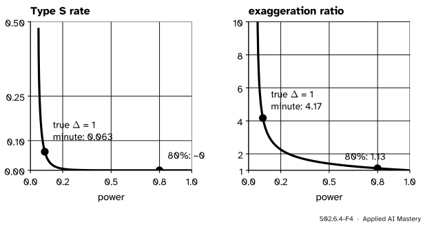
Gelman and Carlin named these failures. A Type M error (magnitude) is a significant estimate that exaggerates the effect; the exaggeration ratio is the expected size of a significant estimate divided by the true effect. A Type S error (sign) is a significant estimate with the wrong sign. Both are small when power is high and severe when power is low.
Build it up
Step 1. Power by simulation. A formula exists for few tests. A simulation works for every test: draw samples from the alternative, run the test, count the rejections. The share of rejections estimates the power.
Step 2. Check it where a formula exists. For the designs (\(\delta = 1.095\), five per group) the noncentral t gave 0.333 (S02.6.3). The simulation should agree within its own sampling error.
Step 3. Use it where none does. The Mann-Whitney test (S02.7.4) on the same alternative has no handy power formula. The simulation answers in the same few lines.
Step 4. Look at what survives. Keep the estimates as well as the decisions. Among the rejections, measure the average size and count the wrong signs.
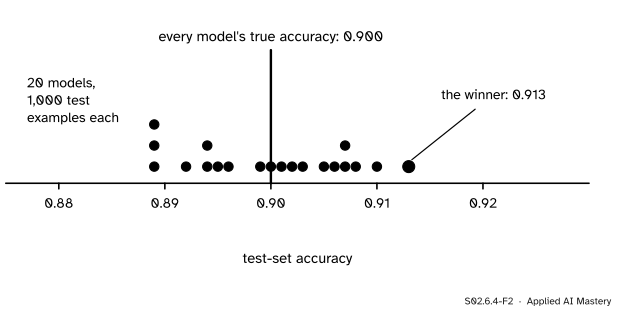
Step 5. Selection is the same everywhere. A leaderboard reports the best of many models scored on one test set. If all of them are equally good, the winner is simply the luckiest.
S02.6.4-F2
The winner’s curse. Twenty models with identical true accuracy 0.900, each scored on 1,000 test examples. The top score, 0.913, is the luckiest draw, not the best model.
The formal statement
Simulated power. Run \(K\) independent simulated experiments under the alternative and let \(R\) be the number that reject. The estimate \(\hat{\pi} = R/K\) is a sample proportion, so its standard error is \({\sqrt{\pi(1-\pi)/K}}\) (S02.1.2). For \(\pi = 0.333\) and \(K = 20{,}000\) that is 0.0033: enough for two decimals.
NoteDefinitions: design analysis (Gelman and Carlin)
Let \(\hat{D}\) be an estimate of a true effect \(D > 0\), judged significant when it is far enough from zero. Then
power\(= \Prob(\text{significant})\);
Type S rate\(= \Prob(\hat{D} < 0 \mid \text{significant})\);
Why low power exaggerates. Take the simplest case, \(\hat{D}\) normal with mean \(D\) and known standard error \(s\), significant when \({\abs{\hat{D}} > 1.96\,s}\). Every significant estimate is larger than \({1.96\,s}\) in size. If the study has low power, \(D\) is well below \({1.96\,s}\), so every significant estimate overstates \(D\), and the exaggeration ratio is above \({1.96\,s/D}\). For the designs with a true gain of one minute, \(s = {\sqrt{7.5 \times 2/5}} = 1.732\), so significant estimates are at least \({1.96 \times 1.732} = 3.39\) minutes, more than three times the truth. The t-test’s own cut-off varies with the sample’s spread, which blurs the edge, but the simulation shows the same picture.
S02.6.4-F4
Both errors against power, for a normal estimate. Below about 0.5 power the exaggeration grows fast; below about 0.1 the sign itself becomes unreliable.
In the normal model with \(\lambda = D/s\), the power is \({1 - \Phi(1.96 - \lambda) + \Phi(-1.96 - \lambda)}\) and the Type S rate is the second term divided by the power. For \(\lambda = {1/1.732} = 0.577\) these give power 0.089 and Type S rate 0.063; at \(\lambda = 2.8\), power 0.80 and Type S rate \(1.2 \times 10^{-6}\), the values Gelman and Carlin report.
Go deeper: the exaggeration ratio in closed form
Write \(\hat{D} = s(\lambda + Z)\) with \(Z\) standard normal, and let \({a = 1.96 - \lambda}\) and \({b = -1.96 - \lambda}\). Because \({\phi'(z) = -z\phi(z)}\), the tail integral \({\int_a^\infty z\phi(z)\,dz} = \phi(a)\), and \({\int_{-\infty}^b z\phi(z)\,dz} = -\phi(b)\). So
Their sum, divided by \({\text{power} \times D}\), is the exaggeration ratio. It gives 4.17 at \(\lambda = 0.577\) and 1.13 at \(\lambda = 2.8\) (Gelman and Carlin’s simulation reports 1.12).
Observed power adds nothing. “Post hoc” or observed power plugs the observed effect into the power formula after the study. For the one-sided z-test the observed statistic is \({z_{\text{obs}} = \Phi^{-1}(1 - \text{p-value})}\), and using it as the shift \(\lambda\) gives
Since \(z_{\text{obs}}\) is fixed by the p-value, this is a function of the p-value alone. At p-value \(= \alpha\) the bracket is zero and the observed power is exactly 0.5; a larger p-value always means a smaller observed power. Hoenig and Heisey derive this for the z-test and point out that for any test the observed power is a one-to-one function of the p-value.
Worked example
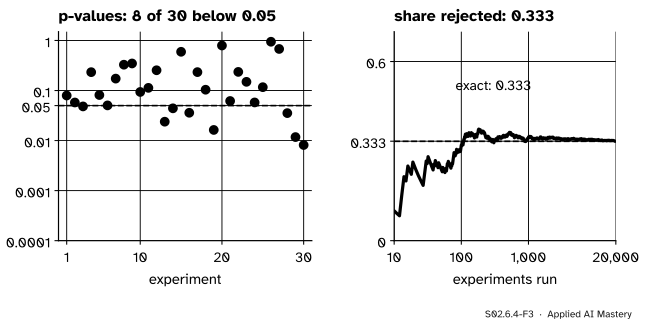
Simulated power for the two designs. Draw five visitors per design from normal populations 3 minutes apart with standard deviation \({\sqrt{7.5}}\), run ttest_ind, and repeat.
S02.6.4-F3
Simulated power, experiment by experiment. Eight of the first 30 reject; after 20,000 the share is 0.333, the noncentral t’s answer.
Of the first 30 experiments, 8 reject: a rough 0.27.
After 20,000, the share is 0.333, against the exact 0.333, with Monte Carlo standard error 0.0033.
The same 20,000 data sets tested with the Mann-Whitney test give 0.24. With five per group its exact p-values jump from 0.032 to 0.056, so it rejects only when \({U \ge 23}\) or \({U \le 2}\) out of 25: rank tests pay for tiny samples.
Type M and S for a true gain of one minute. The same study with a true difference of 1 minute (\(\delta = 0.365\)) has power only 0.08 by the noncentral t. In 20,000 simulated runs about 8 percent reject. Their estimates average about 3.9 minutes in size, an exaggeration ratio near 3.9, and about 7 percent of them point the wrong way. A team that sees “four minutes, p-value 0.03” from five visitors per design has learnt that the effect is probably positive, and almost nothing about its size.
Code
From scratch with NumPy, vectorised over 20,000 experiments:
import mathimport numpy as npfrom scipy import statssigma = math.sqrt(7.5)def simulate(true_diff, n=5, reps=20_000, seed=4): rng = np.random.default_rng(seed) a = rng.normal(7, sigma, size=(reps, n)) b = rng.normal(7+ true_diff, sigma, size=(reps, n))return a, ba, b = simulate(3.0)p_t = stats.ttest_ind(b, a, axis=1).pvaluep_u = stats.mannwhitneyu(b, a, axis=1, method="exact").pvaluepower_t, power_u = np.mean(p_t <0.05), np.mean(p_u <0.05)mc_se = math.sqrt(power_t * (1- power_t) /len(p_t))print(f"t-test {power_t:.3f} (Monte Carlo SE {mc_se:.4f}), Mann-Whitney {power_u:.3f}, first 30: {np.sum(p_t[:30] <0.05)}")
t-test 0.333 (Monte Carlo SE 0.0033), Mann-Whitney 0.243, first 30: 8
The library call is scipy.stats.power. Its significance defaults to 0.01, so pass 0.05:
Type M and Type S errors, simulated for a true gain of one minute:
a, b = simulate(1.0, seed=6)estimates = b.mean(axis=1) - a.mean(axis=1)significant = stats.ttest_ind(b, a, axis=1).pvalue <0.05print(f"power {significant.mean():.3f}")print(f"exaggeration ratio {np.abs(estimates[significant]).mean() /1.0:.2f}")print(f"Type S rate {np.mean(estimates[significant] <0):.3f}")
power 0.079
exaggeration ratio 3.88
Type S rate 0.070
The winner’s curse: twenty models with true accuracy 0.900 on 1,000 test examples each, one leaderboard and then 20,000 of them:
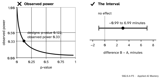
p-value 0.122, observed power 0.33
one-sided z, p-value 0.05: 0.5
Explore
The module’s interactive, the power explorer, is in lesson S02.6.1. Set \(\delta = 0.365\) (a one-minute gain for the designs) and \(n = 5\): the power reads about 0.09, the regime where the exaggeration ratio in the figure above is about four.
Pitfalls
S02.6.4-F5
Wrong beside right after a non-significant result. Observed power only restates the p-value. The interval shows which effects the data leave open: from about a one-minute loss to a seven-minute gain.
“Not significant, but observed power was only 0.33, so the study was too small and the effect is real.”
Observed power is a re-expression of the p-value 0.122, so it cannot add evidence. Power belongs before a study, computed for an effect worth finding. After it, report the interval, \(-0.99\) to \(6.99\) minutes.
“Significant despite a tiny sample, so the effect must be big.”
That is exactly when Type M errors are worst: with power 0.08, significant estimates are about four times the truth. A surprising, significant result from a small study needs replication, not celebration.
“Our model tops the leaderboard, so it is the best.”
Out of many similar models scored on one test set, the top score includes the most luck: twenty equal models on 1,000 examples produce a winner about 1.7 points above the truth on average. Re-evaluate the chosen model on fresh data (ML01.9) and correct for the comparisons made (S02.9).
“scipy.stats.power tests at 0.05.”
Its significance defaults to 0.01. Leave it out and you simulate a stricter test with less power.
Check yourself
Recall
1. How is power estimated by simulation?
Show answer
Draw many data sets from the alternative, run the test on each, and take the share that reject.
2. What is a Type M error, and what is the exaggeration ratio?
Show answer
A significant estimate that overstates the effect’s size; the ratio is the expected size of a significant estimate divided by the true effect.
3. What is a Type S error?
Show answer
A significant estimate whose sign is opposite to the true effect’s.
4. Why does observed power add nothing to the p-value?
Show answer
It is computed from the observed effect, which the p-value already summarises: observed power is a one-to-one function of the p-value.
5. What is the winner’s curse on a leaderboard?
Show answer
The top score among many similar models is biased upwards, because it is the one with the luckiest test-set error.
Exercises
1.★ A simulation of 20,000 experiments gives power 0.333. What is its Monte Carlo standard error, and how many experiments would bring it to 0.001?
Show solution
\({\sqrt{0.333 \times 0.667/20{,}000}} = 0.0033\). For 0.001 we need \({K = 0.333 \times 0.667/0.001^2} \approx 222{,}000\) experiments.
2.★★ An estimate is normal with standard error \(s\) and the true effect is \(D = s\). At level 0.05 two-sided, find the power and the Type S rate.
Show solution
\(\lambda = 1\). Power \({= 1 - \Phi(1.96 - 1)} + \Phi(-1.96 - 1)\), which is \({0.1685 + 0.0015} = 0.170\). The Type S rate is \({0.0015/0.170} = 0.009\): rare, but the exaggeration ratio here is about 2.5.
3.★★★ For the one-sided z-test at level \(\alpha\), show that a non-significant result always has observed power below one half.
Show solution
Observed power is \({1 - \Phi(z_{1-\alpha} - z_{\text{obs}})}\). Not significant means \({z_{\text{obs}} < z_{1-\alpha}}\), so the argument \({z_{1-\alpha} - z_{\text{obs}}}\) is positive and \({\Phi(\cdot)} > \tfrac12\), which makes the observed power less than \(\tfrac12\). “Low observed power” after a non-significant result is therefore guaranteed, and says nothing.
Summary card
Low power does not only miss effects; it distorts the ones it finds.
S02.6.4-F1
The significance filter.
Simulated power. Share of rejections under the alternative; SE \({\sqrt{\pi(1-\pi)/K}}\).
Type M. Significant estimates exaggerate when power is low.
Type S. Below about 0.1 power, signs become unreliable.
Observed power. A function of the p-value; report the interval instead.
Sources and next steps
Sources. Each was opened and checked against this lesson on 15 November 2026.
Andrew Gelman and John Carlin, Beyond power calculations: assessing Type S (sign) and Type M (magnitude) errors, Perspectives on Psychological Science 9(6), 641–651, 2014. Defines power, the Type S error rate and the exaggeration ratio for a hypothetical replication; for a normal estimate 2.8 standard errors from zero reports power 0.80, Type S rate \({1.2 \times 10^{-6}}\) and exaggeration factor 1.12, and its Figure 2 plots both errors against power.
SciPy, scipy.stats.power. Simulates the power of a test under an alternative; significance defaults to 0.01 and n_resamples to 10,000.
Next. Module S02.7, Common tests, names the tests whose power this module has been computing, and S05.3 plans the length of A/B tests with the same formulas.