A two-sided test rejects a null value exactly when it lies outside the confidence interval, so an interval is the set of values the data do not reject. Then separate statistical from practical significance, and see how running many analyses inflates false positives.
S02.5.4L2 Intermediate25 minIn review (what this means)
The maths and code on this page are checked by automated tests on every change, but an independent reader has not signed it off yet. Spot a mistake or a confusing step? Tell us.
Derive that a two-sided level-alpha test rejects mu_0 exactly when mu_0 lies outside the 1 - alpha confidence interval.
Read a confidence interval as the set of null values the data do not reject, using design A’s interval 3.60 to 10.40.
Tell statistical from practical significance, and report an estimate with its interval rather than a p-value alone.
Show by simulation that reporting the best of several analyses inflates the false-positive rate.
The question
One team reports that its model beats a baseline accuracy of 0.900 “with a p-value below \({10^{-20}}\)”. Another reports a gain of 3 points “that was not significant”. Which result should change what you do next? And is a confidence interval a different tool from a test, or the same tool held the other way round?
From the last lesson
1. What is a Type I error, and what is its probability in a level-\(\alpha\) test?
Show answer
Rejecting \(H_0\) when it is true; its probability is \(\alpha\).
2. Write the critical value of the one-sided z-test on the scale of \(\bar{x}\), and its value for the listing site at \({\alpha = 0.05}\).
Show answer
\({c}\)\({= \mu_0 + z_{1-\alpha}\,\sigma/\sqrt{n}}\), which is \({8.3 + 1.645 \times 1.082 = 10.08}\).
Intuition
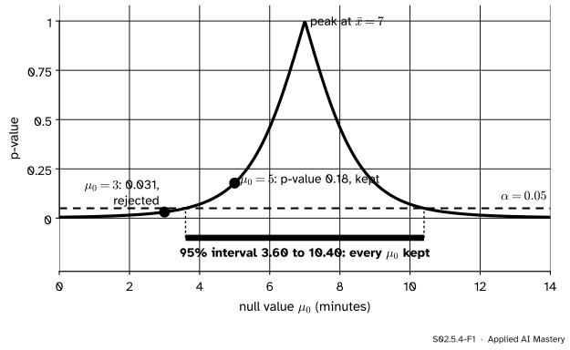
Take design A from S02.4 (invented): five visitors spent 4, 5, 7, 8 and 11 minutes on a page, with mean 7. Instead of testing one null value, test them all. For every candidate mean \(\mu_0\), run the two-sided t-test and plot its p-value.
S02.5.4-F1
Every null value tested at once. The values whose p-value stays above 0.05 form an unbroken stretch, and that stretch is exactly the 95 percent t-interval of S02.4, 3.60 to 10.40.
The p-value is 1 at \({\mu_0 = 7}\), where the data sit exactly on the null value, and it falls the further \(\mu_0\) moves away. Cut the curve at \({\alpha = 0.05}\). The null values that survive are those from 3.60 to 10.40, and that is the confidence interval. An interval is the set of null values that the data do not reject.
Build it up
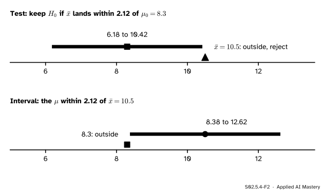
Step 1. One test, one null value. For the listing site of the last two lessons, the two-sided z-test keeps \({\mu_0 = 8.3}\) when \(\bar{x}\) lies within \({1.96 \times 1.082 = 2.12}\) of 8.3.
Step 2. Read the distance the other way. “\(\bar{x}\) is within 2.12 of \(\mu_0\)” says the same as “\(\mu_0\) is within 2.12 of \(\bar{x}\)”. The set of \(\mu_0\) within 2.12 of \({\bar{x} = 10.5}\) is \({10.5 \pm 2.12}\), from 8.38 to 12.62: the 95 percent z-interval of S02.4.1.
S02.5.4-F2
The same gap of 2.2 measured from either end. It is more than 2.12, so the test rejects 8.3 and the interval leaves 8.3 out. The two verdicts can never disagree.
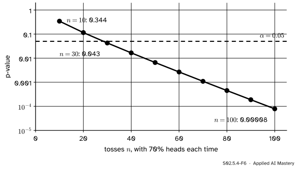
Step 3. Statistically significant is not the same as important. A result is statistically significant when its p-value is below \(\alpha\); it is practically significant when the effect is large enough to matter. The p-value cannot tell the two apart, because it mixes the size of the effect with the amount of data. Keep the coin’s proportion of heads at 0.7 and toss more and more often.
S02.5.4-F6
The same effect, 0.7 heads against a fair 0.5, at ten sample sizes. The p-value falls from 0.344 at ten tosses to 0.00008 at a hundred. Nothing about the coin changed; only the amount of data.
Turn it round. Any effect, however small, becomes “significant” with enough data. A model with accuracy 0.901 on 10 million test examples beats a baseline of exactly 0.900 with \({z = 10.5}\) and a p-value near \({10^{-25}}\). The gain is a tenth of a point.
The formal statement
NoteTheorem: tests and intervals are one object
For data with known \(\sigma\), the two-sided level-\(\alpha\) z-test rejects \({H_0 : \mu = \mu_0}\) exactly when \(\mu_0\) lies outside the \({1 - \alpha}\) confidence interval
The same holds for the t-test and the t-interval, with \({t_{n-1,\,1-\alpha/2}}\) and \({s/\sqrt{n}}\).
Proof. Write \({\mathrm{SE} = \sigma/\sqrt{n}}\) and \({q = z_{1-\alpha/2}}\). From the last lesson, the test keeps \(H_0\) exactly when \({\abs{z} < q}\). Each line below is the same condition:
The first step is the test’s rule, the second multiplies by the positive SE, the third uses \({\abs{a - b} = \abs{b - a}}\), and the fourth unpacks the absolute value. The last line says \(\mu_0\) is inside the interval. For the t-test replace \(q\) by \({t_{n-1,\,1-\alpha/2}}\) and SE by \({s/\sqrt{n}}\); nothing else changes. At an end of the interval the p-value is exactly \(\alpha\), the boundary case. ∎
The theorem can be taken as a definition: the \({1 - \alpha}\) confidence interval is the set of null values a level-\(\alpha\) test does not reject. Read that way, an interval carries more than a p-value. It says which values are ruled out, which are not, and how wide the uncertainty is.
S02.5.4-F4
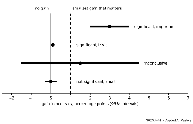
Four invented results, each a 95 percent interval for a gain. Only the interval shows which “significant” result matters and which “not significant” result is informative.
Each interval answers two questions that a p-value lumps together. Does it exclude 0? That is statistical significance. Does it clear the smallest gain that matters, here 1 point? That is practical significance. The third result is not “no effect”: it allows a loss of 1.5 points and a gain of 4.5. The fourth is informative: whatever the gain is, it is small. So report the estimate and its interval, not only a p-value. The ASA’s statement on p-values makes the same point.
Worked example
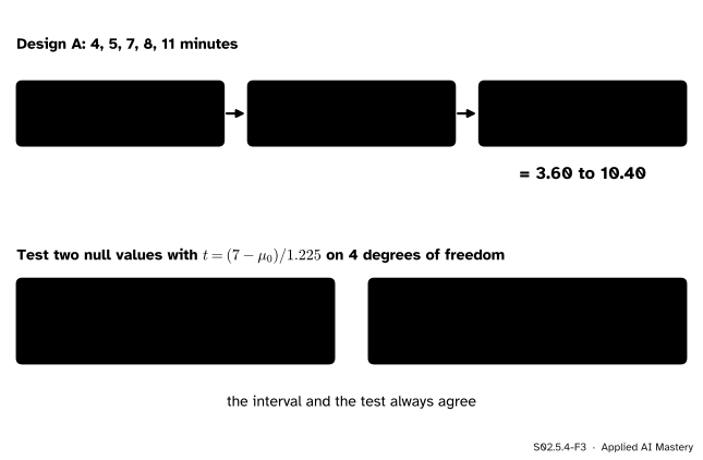
Design A: which null values of the mean time on the page do the data reject?
S02.5.4-F3
One interval, two tests. The test of 5 keeps it and 5 is inside; the test of 3 rejects it and 3 is outside.
Interval.\({\bar{x} = 35/5 = 7}\). The squared deviations are 9, 4, 0, 1 and 16, which add to 30, so \({s^2 = 30/4 = 7.5}\) and \({s = 2.739}\). Then \({s/\sqrt{5} = 1.225}\), and with \({t_{4,\,0.975} = 2.776}\) the margin is \({2.776 \times 1.225 = 3.40}\). The 95 percent interval is \({7 \pm 3.40}\), from 3.60 to 10.40.
Test \({\mu_0 = 5}\).\({t = (7 - 5)/1.225 = 1.63}\) on 4 degrees of freedom; the two-sided p-value is 0.178, above 0.05, so 5 is kept. It lies inside the interval, as the theorem demands.
Test \({\mu_0 = 3}\).\({t = (7 - 3)/1.225 = 3.27}\), p-value 0.031, below 0.05, so 3 is rejected. It lies outside the interval.
At the edge.\({\mu_0 = 3.60}\) gives \({t = 2.776}\) and a p-value of exactly 0.05 (to rounding). Every value from 3.60 to 10.40 is compatible with the five times; with only five visitors that is a wide range, and that width is the honest summary.
Code
From scratch: test a fine grid of null values and keep those the t-test does not reject. The ends of the kept stretch should be the ends of the t-interval.
import mathimport numpy as npfrom scipy import statsa = np.array([4, 5, 7, 8, 11.0])n, xbar, s =len(a), a.mean(), a.std(ddof=1)se = s / math.sqrt(n)t975 = stats.t.ppf(0.975, df=n -1)def p_two_sided(mu0):return2* stats.t.sf(abs((xbar - mu0) / se), df=n -1)grid = np.round(np.arange(0, 14.0001, 0.01), 2)kept = grid[[p_two_sided(m) >=0.05for m in grid]]print(f"x-bar {xbar}, s {s:.3f}, se {se:.3f}, t quantile {t975:.3f}")print(f"kept null values run from {kept.min():.2f} to {kept.max():.2f}")print(f"t-interval: {xbar - t975 * se:.2f} to {xbar + t975 * se:.2f}")print(f"p-values: mu0 = 5 -> {p_two_sided(5):.3f}, mu0 = 3 -> {p_two_sided(3):.3f}")
x-bar 7.0, s 2.739, se 1.225, t quantile 2.776
kept null values run from 3.60 to 10.40
t-interval: 3.60 to 10.40
p-values: mu0 = 5 -> 0.178, mu0 = 3 -> 0.031
The grid’s ends, 3.60 and 10.40, are the interval’s ends. The library gives both views from one call: ttest_1samp returns the test and its confidence_interval() method the interval.
res = stats.ttest_1samp(a, popmean=5)ci = res.confidence_interval(confidence_level=0.95)print(f"t = {res.statistic:.3f}, p-value {res.pvalue:.3f}, 95% interval {ci.low:.2f} to {ci.high:.2f}")# statistical against practical significance: 0.901 against 0.900 on ten million examplesn_big =10_000_000z_big = (0.901-0.900) / math.sqrt(0.900*0.100/ n_big)print(f"z = {z_big:.1f}, two-sided p-value {2* stats.norm.sf(z_big):.1e}")
t = 1.633, p-value 0.178, 95% interval 3.60 to 10.40
z = 10.5, two-sided p-value 5.6e-26
Last, the danger of many analyses. Simulate 20,000 studies in which nothing is going on, each measuring five unrelated outcomes, and report the smallest of the five p-values.
rng = np.random.default_rng(11)z = rng.standard_normal((20_000, 5)) # every H0 truepvals =2* stats.norm.sf(np.abs(z))best = pvals.min(axis=1)print(f"one planned outcome below 0.05: {np.mean(pvals[:, 0] <=0.05):.3f}")print(f"best of five below 0.05: {np.mean(best <=0.05):.3f}")
one planned outcome below 0.05: 0.048
best of five below 0.05:       0.224
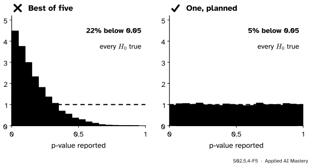
One planned outcome gives a false positive 5 percent of the time, as promised. Picking the best of five gives one about 22 percent of the time. Module S02.9 derives the exact rate and the corrections that restore the promise.
Explore
This module’s interactive, the p-value machine, is in lesson S02.5.2. Use it to see the effect of sample size from this lesson: keep the observed share of heads at 0.7 (7 of 10, then 14 of 20, then 21 of 30) and watch the two-sided p-value fall from 0.344 towards 0.043, with the effect unchanged.
Pitfalls
S02.5.4-F5
Wrong beside right. Reporting the best of five analyses turns a 5 percent false-alarm rate into about 22 percent; one analysis fixed in advance keeps it at 5 percent.
“Significant, so it matters.”
Significance says the data are hard to explain with the null value; it says nothing about size. With 10 million examples a gain of 0.1 points is overwhelmingly significant and practically nothing. Report the estimate and its interval, and compare the interval with the smallest effect that would change a decision.
“Not significant, so there is no effect.”
A wide interval that includes 0 also includes large effects. The two page designs of S02.4.4 differ by 3 minutes, a big change for a web page, with a 95 percent interval from −0.99 to 6.99: not significant at 0.05, yet far from showing that the designs are equal.
“I tried a few analyses and reported the one that worked.”
Each extra analysis is another chance for a false alarm. Trying outcomes, subgroups, ways of handling outliers or transformations until one gives a p-value below 0.05 inflates the real false-positive rate far above 5 percent, as the simulation shows; the ASA’s release on its statement calls this p-hacking. In machine learning the same thing happens when many models are tried on one validation set and the best score is reported (ML01.9.4). Fix the analysis in advance, or correct for the number of tests (S02.9).
Check yourself
Recall
1. State the link between a two-sided level-\(\alpha\) test and the \({1 - \alpha}\) confidence interval.
Show answer
The test rejects \({\mu_0}\) exactly when \({\mu_0}\) lies outside the interval; the interval is the set of null values the test does not reject.
2. Design A’s 95 percent interval is 3.60 to 10.40. Without computing, is \({\mu_0 = 11}\) rejected at level 0.05?
Show answer
Yes: 11 lies outside the interval. (Its p-value is 0.031.)
3. What is the difference between statistical and practical significance?
Show answer
Statistical significance means the p-value is below \(\alpha\); practical significance means the effect is large enough to matter. Large samples make tiny effects statistically significant.
4. Why does the p-value for 70 percent heads fall as the number of tosses grows?
Show answer
The standard error shrinks like \({1/\sqrt{n}}\), so the same gap of 0.2 from 0.5 becomes more and more standard errors wide.
5. In the simulation, what false-positive rate did “best of five analyses” give, against the promised 5 percent?
Show answer
About 22 percent.
Exercises
1.★ Using only design A’s interval, 3.60 to 10.40, decide at level 0.05 whether each null value is rejected: \({\mu_0 = 4}\), \({\mu_0 = 10}\), \({\mu_0 = 11}\).
Show solution
4 and 10 are inside, so they are kept (their p-values are both 0.070). 11 is outside, so it is rejected (p-value 0.031).
2.★★ For the listing site (\({\bar{x} = 10.5}\), \({\mathrm{SE} = 1.082}\)), build the 99 percent z-interval with \({z_{0.995} = 2.576}\). Is 8.3 inside? Check that this agrees with the two-sided p-value 0.042.
Show solution
The margin is \({2.576 \times 1.082 = 2.787}\), so the interval is \({10.5 \pm 2.787}\), from 7.71 to 13.29. It contains 8.3, so a level-0.01 test keeps \({\mu_0 = 8.3}\). That agrees with the p-value: 0.042 is above 0.01. At level 0.05 the 95 percent interval, 8.38 to 12.62, leaves 8.3 out, and 0.042 is below 0.05. Both pairs agree, as the theorem says they must.
3.★★★ A model’s accuracy is compared with a baseline of 0.900, with per-example standard deviation \({\sqrt{0.9 \times 0.1} = 0.3}\). Show that the two-sided z statistic for a true gain \(\Delta\) on \(n\) examples is about \({\Delta\sqrt{n}/0.3}\), and find how many examples make a gain of 0.001 significant at level 0.05.
Show solution
The observed accuracy has standard error \({0.3/\sqrt{n}}\) under \(H_0\), so if it comes out at \({0.900 + \Delta}\),
\[
z = \frac{\Delta}{0.3/\sqrt{n}} = \frac{\Delta\sqrt{n}}{0.3} .
\]
The test rejects when \({z \ge 1.96}\), that is when
About 346,000 test examples make a tenth of a point significant. Because \(z\) grows like \({\sqrt{n}}\), every nonzero gain becomes significant for large enough \(n\); significance alone cannot say whether the gain is worth having.
Summary card
An interval is the set of null values the data do not reject, and it shows size as well.
S02.5.4-F1
Cut the p-value curve at \(\alpha\).
Duality. Reject \({\mu_0}\) at level \(\alpha\) exactly when \({\mu_0}\) is outside the \({1 - \alpha}\) interval.
Significance is not importance.\(z\) grows like \({\sqrt{n}}\); report the estimate and its interval.
Many analyses. The best of five null p-values is below 0.05 about 22 percent of the time.
Sources and next steps
Sources. Each was opened and checked against this lesson on 15 November 2026.
Jeremy Orloff and Jonathan Bloom, Reading 23a, Confidence Intervals: Three Views, MIT OpenCourseWare 18.05 (Spring 2022). Section 4, confidence intervals via hypothesis testing, defines the \({(1 - \alpha)}\) interval as all values \({\theta_0}\) not rejected at level \(\alpha\) when they are the null hypothesis.
David Diez, Mine Cetinkaya-Rundel and Christopher Barr, OpenIntro Statistics, fourth edition (free PDF). Section 5.3.2 tests hypotheses by checking whether the null value lies in a confidence interval, and Section 5.3.6 separates statistical from practical significance.
American Statistical Association, press release on its Statement on Statistical Significance and P-Values, 7 March 2016. Principle 3: decisions should not rest only on whether a p-value passes a threshold; principle 4: proper inference requires full reporting and transparency; principle 5: a p-value does not measure the size of an effect. In it the ASA’s president names the practices called p-hacking and data dredging.
SciPy developers, scipy.stats.ttest_1samp: the arguments popmean and alternative, the result’s statistic, pvalue and df, and its confidence_interval method, whose confidence_level is 0.95 by default.
Next. S02.6 asks how likely a test is to detect an effect of a given size (its power) and how much data that takes. S02.7 runs the named tests, and S02.9 corrects for testing many hypotheses.