When the population’s spread is unknown, estimate it from the sample and widen the multiplier from 1.96 to a t quantile. Build the t-interval for design A’s five times, then test its promise by simulation on normal and on skewed data.
S02.4.2L2 Intermediate25 minIn review (what this means)
The maths and code on this page are checked by automated tests on every change, but an independent reader has not signed it off yet. Spot a mistake or a confusing step? Tell us.
Derive the t-interval from the pivot (x-bar minus mu) over (s / sqrt(n)) and its t distribution with n - 1 degrees of freedom.
Compute a 95 percent t-interval by hand, by NumPy and with scipy.stats.t.interval and ttest_1samp.
Explain why 1.96 with s in place of sigma covers too rarely for small samples.
Check coverage by simulation and describe how the t-interval falls short for small samples from a skewed population.
The question
Five visitors shown design A spent 4, 5, 7, 8 and 11 minutes on the page. Nobody knows the spread of such times across all visitors; all we have is these five. How wide must an honest 95 percent interval for the mean time be, and what does it cost us not to know \(\sigma\)?
From the last lesson
1. How does the width of a z-interval change when the sample size is multiplied by four?
Show answer
It halves: the width is proportional to \({1 / \sqrt{n}}\).
2. A 95 percent interval came out as 6.65 to 10.89. What does the 95 percent describe?
Show answer
The method: in repeated samples, 95 percent of the intervals it makes cover the true mean. This one interval either covers it or not.
Intuition
The z-interval of the last lesson needed the population’s standard deviation \(\sigma\). Outside an invented city we do not have it, so we put the sample’s own standard deviation \(s\) in its place. But \(s\) is itself a guess, and from five numbers a shaky one: some samples make it too small, and then the interval is too narrow exactly when it most needs to be wide.
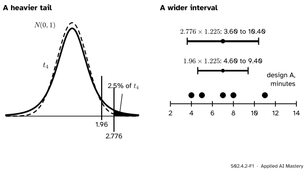
The fix is to widen the multiplier. With \(s\) in the formula, the standardised mean follows the t distribution (S02.1.4), whose tails are heavier than the normal’s. Its 97.5 percent point for four degrees of freedom is 2.776, not 1.96.
S02.4.2-F1
Left: the \(t_4\) curve has heavier tails, so its 2.5 percent point sits at 2.776 instead of 1.96. Right: for design A the honest interval is therefore 3.60 to 10.40, not 4.60 to 9.40.
The price of not knowing \(\sigma\) is the gap between the two bars: about 40 percent more width for five observations. With more data \(s\) settles down and the price falls.
Build it up
Step 1. Estimate the standard error. Replace \(\sigma\) by \(s\), the standard deviation with divisor \(n - 1\) (S01.3.3, S02.2.1). The estimated standard error is \(\widehat{\mathrm{se}} = {s / \sqrt{n}}\).
Step 2. Ask what the new ratio does. For a normal population, S02.1.4 stated that
where capital \(S\) is the sample standard deviation before we draw. Its distribution involves no unknown parameter, so \(T\) is a pivot, just as \(Z\) was.
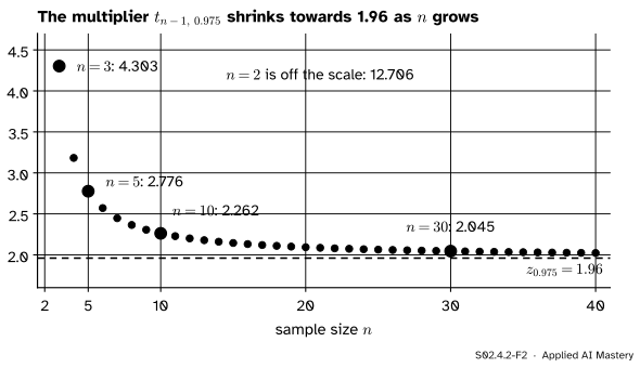
Step 3. Pick the multiplier from that distribution. The middle 95 percent of \(t_{n-1}\) runs from \({-t_{n-1,\,0.975}}\) to \({t_{n-1,\,0.975}}\). That quantile is large for tiny samples and falls towards 1.96 as \(n\) grows, because \(s\) becomes a better stand-in for \(\sigma\).
S02.4.2-F2
The multiplier \({t_{n-1,\,0.975}}\) against \(n\). It is 2.776 for five observations, 2.045 for thirty, and approaches the normal’s 1.96.
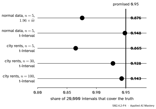
Step 4. Check the promise. For normal data the t-interval covers \(\mu\) in exactly 95 percent of samples. For other populations it relies on the central limit theorem, so we check by simulation.
S02.4.2-F4
Simulated coverage of 95 percent intervals. For normal data the t-interval keeps its promise and 1.96 does not. For the right-skewed city the t-interval falls short at \(n = 5\) and recovers slowly.
The formal statement
NoteThe t-interval for a mean
Let \(x_1, \dots, x_n\) be independent draws from a normal population with unknown mean \(\mu\) and unknown standard deviation \(\sigma\). A \(1 - \alpha\) confidence interval for \(\mu\) is
Its coverage is exactly \(1 - \alpha\) for normal data, and approximately \(1 - \alpha\) for other populations when \(n\) is large enough for the central limit theorem.
Derivation. It follows the four lines of the z-interval with \(S\) in place of \(\sigma\). Write \(q = {t_{n-1,\,0.975}}\) and \(\widehat{\mathrm{SE}} = {S / \sqrt{n}}\). By Step 2, this event has probability 0.95:
The only change from the z-interval is that the multiplier now accounts for the randomness of \(S\) as well as of \(\bar{X}\).
Why 1.96 with \(s\) falls short. Using 1.96 with \(s\) means claiming \({\Prob(\abs{T} \le 1.96)} = 0.95\). For \(n = 5\) the true value is \({\Prob(\abs{T_4} \le 1.96)} = 0.878\), so about 12 intervals in 100 miss, not 5. The simulation gives 0.876.
Why skewness hurts. For the city, samples of five that miss the few dear Centre flats have both a low mean and a small \(s\), so their intervals are short and sit too low. The two errors line up instead of cancelling. In the simulation 13.2 percent of t-intervals at \(n = 5\) lie wholly below \(\mu\) and only 0.3 percent wholly above. At \(n = 30\) coverage is 0.928, at \(n = 100\) it is 0.943.
Go deeper: an interval for the variance from the chi-square distribution
For a normal population, S02.1.4 stated that \({(n - 1) S^2 / \sigma^2} \sim \chi^2_{n-1}\), another pivot. Its middle 95 percent runs from \({\chi^2_{n-1,\,0.025}}\) to \({\chi^2_{n-1,\,0.975}}\), so this event has probability 0.95:
For design A, \({(n - 1)s^2} = 30\), and \({\chi^2_{4,\,0.025}} = 0.484\), \({\chi^2_{4,\,0.975}} = 11.143\). The interval for \(\sigma^2\) is \({30 / 11.143} = 2.69\) to \({30 / 0.484} = 61.93\), and for \(\sigma\) its square roots, 1.64 to 7.87. Five points say very little about a spread. Unlike the t-interval this one is not symmetric about \(s^2 = 7.5\), because the chi-square distribution is not symmetric, and it leans on normality much more heavily than the t-interval does.
Worked example
Design A’s five times: 4, 5, 7, 8, 11 minutes.
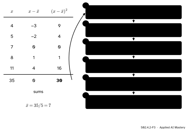
S02.4.2-F3
The t-interval for design A, step by step.
Mean.\({35 / 5} = 7\).
Squared deviations.\(9 + 4 + 0 + 1 + 16 = 30\). The deviations themselves add to 0, a useful check.
Variance and standard deviation.\(s^2 = {30 / 4} = 7.5\) and \(s = {\sqrt{7.5}} = 2.739\).
Multiplier.\(n - 1 = 4\) degrees of freedom, so \({t_{4,\,0.975}} = 2.776\).
Margin and interval.\({2.776 \times 1.225 = 3.40}\), and \(7 \pm 3.40\) runs from 3.60 to 10.40 minutes.
Had we used 1.96, the margin would be 2.40 and the interval 4.60 to 9.40, about 30 percent narrower and dishonestly so.
Code
From scratch first. Only the quantile comes from SciPy.
import mathimport numpy as npfrom scipy import statsa = np.array([4, 5, 7, 8, 11], dtype=float)n =len(a)xbar = a.sum() / ns = math.sqrt(((a - xbar) **2).sum() / (n -1))se = s / math.sqrt(n)q = stats.t.ppf(0.975, n -1)print(f"x-bar {xbar}, s^2 {s**2:.2f}, s {s:.3f}, se {se:.3f}, t {q:.3f}")print(f"t-interval: {xbar - q * se:.2f} to {xbar + q * se:.2f}")print(f"1.96 with s: {xbar -1.96* se:.2f} to {xbar +1.96* se:.2f}")
x-bar 7.0, s^2 7.50, s 2.739, se 1.225, t 2.776
t-interval: 3.60 to 10.40
1.96 with s: 4.60 to 9.40
Now the promise, checked by simulation: 20,000 samples each from a normal population (mean 7, standard deviation 3) and from the city of S01, built as in the last lesson.
rng = np.random.default_rng(0)parts = []for mean, size in ((5, 250), (8, 150), (17, 100)): draws = rng.gamma(9.0, 1.0, size) parts.append(draws * mean / draws.mean())rents = np.concatenate(parts)mu = rents.mean()def coverage(samples, truth, mult):"""Share of intervals covering the truth, and shares lying wholly below and wholly above it.""" k = samples.shape[1] centre = samples.mean(axis=1) half = mult * samples.std(axis=1, ddof=1) / math.sqrt(k)return (np.mean((centre - half <= truth) & (truth <= centre + half)), np.mean(centre + half < truth), np.mean(centre - half > truth))tq =lambda k: stats.t.ppf(0.975, k -1)rng = np.random.default_rng(42)normal5 = rng.normal(7, 3, (20_000, 5))results = {"normal, n=5, 1.96": coverage(normal5, 7, 1.959964),"normal, n=5, t": coverage(normal5, 7, tq(5)),"normal, n=30, t": coverage(rng.normal(7, 3, (20_000, 30)), 7, tq(30))}for k in (5, 30, 100): results[f"city, n={k}, t"] = coverage(rng.choice(rents, (20_000, k)), mu, tq(k))for name, (cov, below, above) in results.items():print(f"{name:18s} coverage {cov:.3f} wholly below {below:.3f} wholly above {above:.3f}")
normal, n=5, 1.96  coverage 0.876   wholly below 0.063   wholly above 0.062
normal, n=5, t     coverage 0.948   wholly below 0.026   wholly above 0.026
normal, n=30, t    coverage 0.951   wholly below 0.025   wholly above 0.024
city, n=5, t       coverage 0.865   wholly below 0.132   wholly above 0.003
city, n=30, t      coverage 0.928   wholly below 0.064   wholly above 0.008
city, n=100, t     coverage 0.943   wholly below 0.042   wholly above 0.015
Finally the library. scipy.stats.t.interval takes the level, the degrees of freedom, the centre and the scale; ttest_1samp returns a result whose confidence_interval() is the same interval.
print(stats.t.interval(0.95, n -1, loc=a.mean(), scale=stats.sem(a)))print(stats.ttest_1samp(a, popmean=0).confidence_interval(confidence_level=0.95))
The interval from ttest_1samp does not depend on popmean: that argument only sets the null value for the test, which S02.5 and S02.7 take up.
Explore
The module’s interactive, the dance of confidence intervals, lives in lesson S02.4.1. Choose the city, set \(n = 5\) and compare the z method (which uses the true \(\sigma\)) with the t method (which uses \(s\)): the t method’s misses pile up on the low side, as in the simulation above.
Pitfalls
S02.4.2-F5
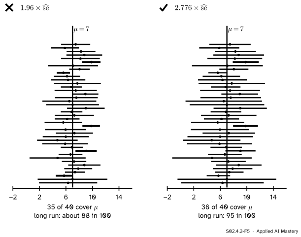
The same forty samples of five. Left: 1.96 with \(s\) misses five times. Right: the t multiplier misses twice, in line with its promise.
“The sample is small, but I can still use 1.96 with \(s\).”
For \(n = 5\) that interval covers only 88 percent of the time. Use \({t_{n-1,\,0.975}}\). The two multipliers are close only for large \(n\) (2.045 against 1.96 at \(n = 30\)), which is why many libraries simply always use \(t\).
“The t-interval makes the normality assumption unnecessary.”
It fixes the cost of estimating \(\sigma\), not the shape of the population. For the skewed city at \(n = 5\) it covers 86.5 percent of the time, with nearly all the misses on one side. Look at the data first (S01.4); for small skewed samples consider a transformation or the bootstrap of S02.8.
“A model’s mean score over five cross-validation folds has a t-interval with four degrees of freedom.”
The t-interval needs independent observations. Cross-validation folds share most of their training data, so their scores are correlated and the interval comes out too narrow. Treat it as a rough guide, not a guarantee.
Check yourself
Recall
1. What changes between the z-interval and the t-interval?
Show answer
\(\sigma\) is replaced by the sample’s \(s\), and the multiplier \(z_{0.975} = 1.96\) by \({t_{n-1,\,0.975}}\).
2. Why is the t multiplier larger than 1.96?
Show answer
Because \(s\) is itself random, the ratio \({(\bar{X} - \mu) / (S / \sqrt{n})}\) varies more than a standard normal: it follows \(t_{n-1}\), whose tails are heavier.
3. What is the 95 percent t-interval for design A?
Show answer
\(7 \pm {2.776 \times 1.225} = 7 \pm 3.40\), from 3.60 to 10.40 minutes.
4. How often does “1.96 with \(s\)” cover the mean for normal samples of five?
Show answer
About 88 percent of the time (\({\Prob(\abs{T_4} \le 1.96)} = 0.878\)), not 95.
5. Why does the t-interval fall short for small samples from the city?
Show answer
The city is skewed to the right. Small samples that miss the dear flats have a low mean and a small \(s\) together, so their intervals are short and too low; at \(n = 5\) coverage is about 0.865.
Exercises
1.★ Design B’s five times are 6, 9, 10, 12, 13. Compute the 95 percent t-interval for its mean.
Show solution
The mean is \({50 / 5} = 10\). The deviations are \(-4, -1, 0, 2, 3\), with squares \(16, 1, 0, 4, 9\) adding to 30, so \(s^2 = {30 / 4} = 7.5\) and \(\widehat{\mathrm{se}} = 1.225\), exactly as for design A. The interval is \(10 \pm 3.40\), from 6.60 to 13.40.
2.★★ How many observations must a normal sample have before \({t_{n-1,\,0.975}}\) is within 0.05 of 1.96? Find the smallest \(n\) with scipy.stats.t.ppf.
Show solution
We need \({t_{n-1,\,0.975}} \le 2.01\). Trying values: at \(n = 49\), \({t_{48,\,0.975}} = 2.011\); at \(n = 50\), \({t_{49,\,0.975}} = 2.0096\). So \(n = 50\) is the smallest. Below about 50 observations the choice between \(t\) and \(z\) changes the width by more than 2.5 percent.
3.★★★ Show that the 95 percent t-interval’s width \({2\,t_{n-1,\,0.975}\,s / \sqrt{n}}\) is itself random, and find its expected value for normal data with \(n = 2\) in terms of \(\sigma\), using \(\E[S] = {\sigma\sqrt{2/\pi}}\) for \(n = 2\).
Show solution
The width depends on \(S\), which changes from sample to sample, so the width is random (unlike the z-interval’s). For \(n = 2\) the multiplier is \({t_{1,\,0.975}} = 12.706\) and \({\sqrt{n}} = {\sqrt{2}}\), so the expected width is
which is about \({14.3\,\sigma}\). The z-interval with known \(\sigma\) would have width \({2 \times 1.96 \times \sigma / \sqrt{2} = 2.77\,\sigma}\). Two observations say very little when the spread is unknown.
Summary card
Not knowing \(\sigma\) costs a wider multiplier, and skewed data cost more.
Design A.\(7 \pm {2.776 \times 1.225}\): 3.60 to 10.40.
Multipliers. 12.706, 2.776, 2.262, 2.045 for \(n = 2, 5, 10, 30\); then towards 1.96.
Promise. Exact for normal data; for skewed data it needs a larger \(n\).
Sources and next steps
Sources. Each was opened and checked against this lesson on 15 November 2026.
Jeremy Orloff and Jonathan Bloom, Reading 22: Confidence intervals based on normal data, MIT OpenCourseWare 18.05, Spring 2022. Section 5.1 defines the t confidence interval with the quantiles of \({t(n - 1)}\), Section 5.2 derives it from the studentised mean, and Section 6 gives the chi-square interval for the variance, noting that it is not symmetric about \(s^2\). The reading names quantiles by the share above them (its \({t_{\alpha/2}}\) is our \({t_{n-1,\,1-\alpha/2}}\)), so its formulas match ours with the subscripts turned round.
scipy.stats.ttest_1samp, SciPy reference: the result’s confidence_interval(confidence_level=0.95) computes a confidence interval around the population mean.