Mean squared error scores an estimator by how far it lands from the truth on average, and splits into bias squared plus variance. See a deliberately biased estimator win, the idea behind ridge, and prove that an MSE that falls to zero makes an estimator consistent.
S02.2.3L2 Intermediate25 minIn review (what this means)
The maths and code on this page are checked by automated tests on every change, but an independent reader has not signed it off yet. Spot a mistake or a confusing step? Tell us.
Derive the decomposition MSE = Bias² + Variance by adding and subtracting the estimator’s mean.
Find the shrinkage factor c that minimises the MSE of c times x-bar, and compute the gain for samples of five city rents.
Show that dividing the sum of squares by n + 1 gives the variance estimate with the smallest MSE for normal data.
Define consistency and prove, with Markov’s inequality, that an estimator whose MSE tends to 0 is consistent.
The question
Ridge regression and weight decay pull a model’s weights towards zero on purpose. The weights are then wrong on average, biased towards zero, and yet the model often predicts new data better. How can a rule that is deliberately wrong on average be closer to the truth than an unbiased one?
From the last lesson
1. Define the efficiency of \(T_1\) relative to \(T_2\).
Show answer
\({\operatorname{Var}(T_2)/\operatorname{Var}(T_1)}\), for two unbiased estimators of the same parameter.
2. What is the efficiency of the median relative to the mean for normal data?
Show answer
\({2/\pi \approx 0.64}\): the median of 157 readings matches the mean of 100.
Intuition
Bias asks where the pile of estimates is centred; variance asks how wide it is. What we usually care about is simpler: how far does an estimate land from the truth, on average? Square the miss, so that misses on either side count alike, and average over samples. That is the mean squared error, and it charges for both faults at once.
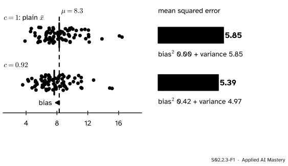
Here is the mean of five city rents, plain and shrunk by a factor 0.92 towards zero.
S02.2.3-F1
Shrinking every estimate by 0.92 moves the centre off the truth, a bias of \({-0.65}\), but narrows the pile. The bias costs 0.42 in squared error and the narrowing saves 0.88, so the mean squared error falls from 5.85 to 5.39.
The shrunk estimates are wrong on average, but each is pulled a little towards zero, and a pile pulled together is narrower. When the pile is wide, as it is for five rents, narrowing it can save more squared error than the small offset costs. That trade, bias for variance, is the subject of this lesson.
Build it up
Take the estimator \({c\bar{X}}\), where the analyst chooses the shrinkage factor\(c\); \({c = 1}\) is the plain mean.
Step 1. Its centre.\({\E[c\bar{X}] = c\mu}\), so \({\text{Bias} = c\mu - \mu = (c - 1)\mu}\).
Step 2. Its spread. Multiplying a random variable by \(c\) multiplies its variance by \(c^2\) (M06.7.3), so \({\operatorname{Var}(c\bar{X}) = c^2\sigma^2/n}\).
Step 3. Its mean squared error. By the decomposition proved in the next section, the MSE is the two added:
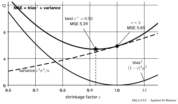
Step 4. Read the curve. Lowering \(c\) from 1 shrinks the variance term at once, while the bias term starts at 0 with zero slope. So a small step below 1 always helps, until the bias term catches up.
S02.2.3-F2
For samples of five city rents, the MSE of \({c\bar{X}}\) is lowest at \({c^* = 0.92}\), not at the unbiased \({c = 1}\).
The formal statement
NoteDefinition: mean squared error
The mean squared error of an estimator \(\hat\theta\) of \(\theta\) is
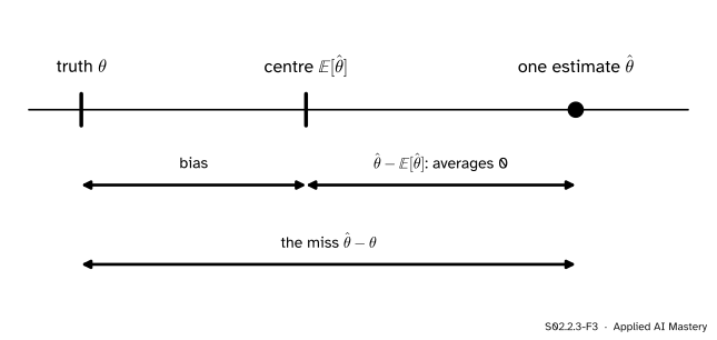
The miss of one estimate is its distance from its own centre plus the bias. The first part changes from sample to sample and averages zero; the second is the same for every sample.
Now average over samples. The first term averages to \({\operatorname{Var}(\hat\theta)}\), by the definition of variance. In the middle term \({\E[\hat\theta] - \theta}\) is a fixed number, so it comes out of the average, leaving \({\E[\hat\theta - \E[\hat\theta]] = \E[\hat\theta] - \E[\hat\theta] = 0}\). The last term is a fixed number, the squared bias. Hence
This is the same split as the bias-variance decomposition of ML01.8.2, where the “estimator” is a fitted model’s prediction and a noise term is added because the target itself is random. For an unbiased estimator the MSE is the variance.
Result 2: the best shrinkage factor. Write \({v = \sigma^2/n}\). Differentiate \({\text{MSE}(c) = c^2 v + (1 - c)^2\mu^2}\) and set the derivative to zero (M04.4):
which is below the plain mean’s \({\sigma^2/n}\) whenever \({\sigma > 0}\). The shrinkage is strongest when the noise \({\sigma^2/n}\) is large beside the signal \(\mu^2\), and \(c^*\) tends to 1 as \(n\) grows. The ridge slope of ML01.9.1 carries a shrinkage factor of the same shape, \({s_{xx}/(s_{xx} + \lambda)}\).
There is a catch: \(c^*\) depends on \(\mu\), the very thing we do not know. So \(c^*\bar{X}\) is not a rule you can apply as it stands. What the calculation proves is that the unbiased mean is never the MSE-best multiple of itself, which is why estimates are so often shrunk in practice, with the amount chosen from the data (by cross-validation for ridge).
Frontier note: shrinking several means at once
With three or more means to estimate together, each from its own normal sample with a known noise variance, Charles Stein showed in 1956 that the separate sample means can be beaten in total MSE, whatever the true means are, and in 1961 James and Stein gave such a rule: shrink all of them towards a common point with a factor computed from the data. Empirical Bayes methods (S04) and the shrinkage inside modern regularised models grow from the same root.
Result 3: the best divisor for a normal variance. For a normal sample, \({\text{SS} = \sum (X_i - \bar{X})^2}\) is \({\sigma^2}\) times a \({\chi^2_{n-1}}\) variable (S02.1.4). A \({\chi^2_k}\) variable is a sum of \(k\) squared standard normals, each with mean 1 and variance \({\E[Z^4] - 1 = 3 - 1 = 2}\), so it has mean \(k\) and variance \({2k}\). Hence \({\E[\text{SS}] = (n-1)\sigma^2}\) and \({\operatorname{Var}(\text{SS}) = 2(n-1)\sigma^4}\). Divide SS by a number \(d\) and write \({a = 1/d}\):
Result 4: if the MSE tends to 0, the estimator is consistent. Markov’s inequality (M06.11.2) says \({\Prob(Y \ge a) \le \E[Y]/a}\) for a variable \({Y \ge 0}\) and \({a > 0}\). Take \({Y = (\hat\theta_n - \theta)^2}\) and \({a = \varepsilon^2}\):
If the MSE tends to 0, so does the right side, and the probability is squeezed to 0. For an unbiased estimator the MSE is the variance and this is Chebyshev’s inequality. Since \({\text{MSE} = \text{Bias}^2 + \operatorname{Var}}\), it is enough that both the bias and the variance tend to 0.
\(\bar{X}\) is consistent: its MSE is \({\sigma^2/n}\). This is the weak law of large numbers again.
The divisor-\(n\) variance is biased but consistent: its bias \({-\sigma^2/n}\) tends to 0, and for normal data its variance \({2(n-1)\sigma^4/n^2}\) does too.
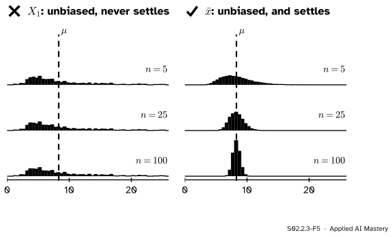
The first observation \(X_1\) alone is unbiased for \(\mu\) and not consistent: it ignores the other \({n - 1}\) values, so its spread never shrinks.
Worked example
For a normal sample of five, which divisor of the sum of squares gives the smallest MSE as an estimate of \(\sigma^2\): 4, 5 or 6?
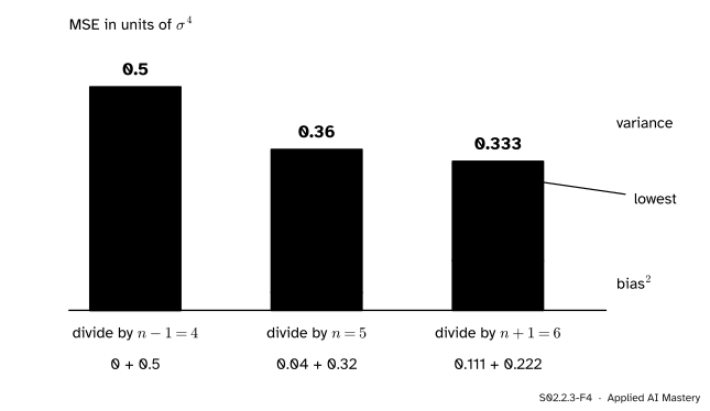
Work in units of \({\sigma^4}\). From Result 3, \({\E[\text{SS}] = 4\sigma^2}\) and \({\operatorname{Var}(\text{SS}) = 8\sigma^4}\).
Divide by 4. Mean \({4/4 = 1}\) times \(\sigma^2\), so bias 0. Variance \({8/16 = 0.5}\). MSE 0.5.
Divide by 5. Mean \({0.8\sigma^2}\), bias \({-0.2\sigma^2}\), bias² 0.04. Variance \({8/25 = 0.32}\). MSE 0.36.
Divide by 6. Mean \({0.667\sigma^2}\), bias² \({(1/3)^2 = 0.111}\). Variance \({8/36 = 0.222}\). MSE 0.333.
S02.2.3-F4
Each step up in the divisor trades variance for bias. The unbiased divisor 4 has the largest MSE; the divisor 6 has the smallest.
The divisor \({n + 1 = 6}\) wins, a third lower than the unbiased choice. This is why “unbiased” is a property to understand, not a goal to chase: for estimating \(\sigma^2\) itself, the textbook \(s^2\) is not the most accurate rule.
Code
First the shrunk mean on samples of five city rents: theory, then simulation.
import numpy as nprng = np.random.default_rng(0) # the city of S01, inventedparts = []for size, mean in [(250, 5.0), (150, 8.0), (100, 17.0)]: draws = rng.gamma(9.0, 1.0, size) parts.append(draws * mean / draws.mean())city = np.concatenate(parts)mu, sigma2, n = city.mean(), city.var(), 5v = sigma2 / nc_star = mu **2/ (mu **2+ v)for c in (1.0, c_star): bias2, var = (1- c) **2* mu **2, c **2* vprint(f"c = {c:.3f}: bias^2 {bias2:.2f} + variance {var:.2f} = MSE {bias2 + var:.2f}")rng = np.random.default_rng(4)xbar = rng.choice(city, size=(20_000, n)).mean(axis=1)print(f"simulated MSE: plain {np.mean((xbar - mu) **2):.2f}, shrunk {np.mean((c_star * xbar - mu) **2):.2f}")
The simulated MSEs sit within a few hundredths of the exact ones. Next the three divisors for normal samples of five, with \({\sigma = 1}\) so that the MSE is in units of \(\sigma^4\).
rng = np.random.default_rng(5)x = rng.normal(0.0, 1.0, (20_000, n))ss = ((x - x.mean(axis=1, keepdims=True)) **2).sum(axis=1)for d in (n -1, n, n +1): theory =2* (n -1) / d **2+ ((n -1) / d -1) **2print(f"divide by {d}: simulated MSE {np.mean((ss / d -1) **2):.3f}, theory {theory:.3f}")
divide by 4: simulated MSE 0.503, theory 0.500
divide by 5: simulated MSE 0.361, theory 0.360
divide by 6: simulated MSE 0.334, theory 0.333
Finally consistency: the chance that \(\bar{X}\) misses \(\mu\) by at least 1, against the bound \({\sigma^2/(n\varepsilon^2)}\) of Result 4.
n =   5: P(|x-bar - mu| >= 1) about 0.683, bound 1.000
n =  25: P(|x-bar - mu| >= 1) about 0.363, bound 1.000
n = 100: P(|x-bar - mu| >= 1) about 0.065, bound 0.293
X_1 alone, any n: 0.864
The bound is loose, 0.293 against about 0.07 at \({n = 100}\), but it falls to 0, which is all a proof of consistency needs. The first observation alone misses by at least 1 with chance 0.864 whatever \(n\) is.
Explore
S02.2-X1
Estimator target
Move the shrinkage factor \(c\) and watch the dots slide and narrow while the bars trade bias² for variance. Then change the sample size \(n\) and see how far the best \(c\) sits from 1.
Three things to try. At \({n = 5}\), press Set c to the best c* and compare the MSE bar with the dashed mark of \({c = 1}\). Drop \(n\) to 2: the best \(c\) falls to 0.82 and shrinking cuts the MSE by 17.5 percent. Raise \(n\) to 50: \(c^*\) is 0.99 and the gain all but vanishes, because \({\sigma^2/n}\) is now tiny beside \({\mu^2 = 68.9}\).
Pitfalls
S02.2.3-F5
Wrong beside right. Both estimators are unbiased at every \(n\). Only the sample mean concentrates on \(\mu\) as \(n\) grows; the first observation alone is as spread at \({n = 100}\) as at \({n = 5}\).
“Unbiased estimators are consistent.”
Unbiasedness is about the centre at one \(n\); consistency is about the whole pile closing in as \(n\) grows. \(X_1\) is unbiased and never closes in. The converse fails too: the divisor-\(n\) variance is biased at every \(n\) and still consistent.
“A biased estimator is a worse estimator.”
Only if bias is all you score. By MSE, \({0.92\bar{X}}\) beats \(\bar{X}\) for five city rents, and the divisor \({n + 1}\) beats \({n - 1}\) for a normal variance. Ridge, weight decay and early stopping all accept bias to cut variance.
“So multiply every mean by \(c^*\).”
\(c^*\) contains the unknown \(\mu\). Plugging \(\bar{X}\) in for \(\mu\) gives a different estimator, with its own bias and variance, that is not guaranteed to win. The lesson of \(c^*\) is that a good amount of shrinkage exists; finding it from data is what validation is for (ML01.9.3).
Check yourself
Recall
1. State the decomposition of the mean squared error.
2. Why does the cross term vanish in its derivation?
Show answer
It is a fixed number, the bias, times \({\hat\theta - \E[\hat\theta]}\), whose average is 0.
3. What shrinkage factor minimises the MSE of \({c\bar{X}}\)?
Show answer
\({c^* = \mu^2/(\mu^2 + \sigma^2/n)}\), which is 0.92 for samples of five city rents.
4. Which divisor of the sum of squares gives the smallest MSE for a normal variance?
Show answer
\({n + 1}\). For \({n = 5}\) the MSEs are 0.5, 0.36 and 0.333 \(\sigma^4\) for divisors 4, 5 and 6.
5. Define consistency, and give a simple condition that guarantees it.
Show answer
\({\Prob(\abs{\hat\theta_n - \theta} \ge \varepsilon) \to 0}\) for every \({\varepsilon > 0}\). It holds whenever \({\text{MSE}(\hat\theta_n) \to 0}\), by Markov’s inequality.
Exercises
1.★ For samples of five city rents, with \({\mu = 8.3}\) and \({\sigma^2/n = 5.85}\), find the MSE of \({0.8\bar{X}}\). Is it better than \(\bar{X}\)?
Show solution
Bias² is \({(1 - 0.8)^2 \times 8.3^2}\), that is \({0.04 \times 68.89 = 2.76}\). Variance is \({0.64 \times 5.85 = 3.74}\). MSE \({= 6.50}\), worse than \(\bar{X}\)’s 5.85: 0.8 shrinks past the best \({c^* = 0.92}\), and the bias now costs more than the variance saves.
2.★★ For normal data, show that the divisor-\(n\) variance estimator has MSE \({(2n - 1)\sigma^4/n^2}\), and conclude that it is consistent.
Show solution
With \({a = 1/n}\) in Result 3, the variance is \({2(n-1)\sigma^4/n^2}\) and the bias is \({\big(\frac{n-1}{n} - 1\big)\sigma^2 = -\sigma^2/n}\), so
For \({n = 5}\) this is \({9/25 = 0.36}\), as in the worked example. It is at most \({2\sigma^4/n}\), which tends to 0, so by Result 4 the estimator is consistent.
3.★★★ Show that the best shrinkage factor satisfies \({c^* < 1}\) for every \({\sigma > 0}\), find it for a single rent, \({n = 1}\), and explain why \({c\bar{X}}\) with a fixed \({c \ne 1}\) is not consistent while \({c^*_n\bar{X}}\) is.
Show solution
\({c^* = \mu^2/(\mu^2 + \sigma^2/n)}\) has a denominator larger than its numerator when \({\sigma^2/n > 0}\), so \({c^* < 1}\). For \({n = 1}\): \({68.89/(68.89 + 29.26) = 0.70}\).
With a fixed \({c \ne 1}\) the bias \({(c - 1)\mu}\) does not depend on \(n\), so (for \({\mu \ne 0}\)) the estimates close in on \({c\mu}\), not on \(\mu\): not consistent. With \({c^*_n}\) the MSE is \({c^*_n\sigma^2/n \le \sigma^2/n}\), which tends to 0, so by Result 4 it is consistent.
Summary card
Score an estimator by its average squared miss: bias² plus variance.
Sources. Each was opened and checked against this lesson on 15 November 2026.
Hossein Pishro-Nik, Introduction to Probability, Statistics, and Random Processes, Section 8.2.1, Evaluating estimators: the definition of the mean squared error, the decomposition \({\text{MSE} = \operatorname{Var} + B^2}\), the definition of a consistent estimator, and the theorem that an MSE tending to 0 gives consistency, proved with Markov’s inequality applied to the squared error.
Wikipedia, Mean squared error: the proof of the bias-variance relationship by adding and subtracting \({\E[\hat\theta]}\); in the section Variance, that for Gaussian data the MSE of the variance estimate is smallest with the divisor \({n + 1}\); and in the section Gaussian distribution the MSEs \({2\sigma^4/(n-1)}\), \({(2n-1)\sigma^4/n^2}\) and \({2\sigma^4/(n+1)}\) for the divisors \({n - 1}\), \(n\) and \({n + 1}\).
Wikipedia, James-Stein estimator, for the frontier block: Stein’s estimator of 1956, simplified by James and Stein in 1961, has lower total MSE than the separate means for every true mean when there are three or more of them and the noise variance is known, and it can be read as an empirical Bayes method.