Three large-sample tests read off one log-likelihood curve: the distance to the null in standard errors, the slope at the null, and the drop from the peak. Run all three on the coin against a fair one, invert them into intervals, and see where they disagree.
S02.10.4L2 Intermediate25 minIn review (what this means)
The maths and code on this page are checked by automated tests on every change, but an independent reader has not signed it off yet. Spot a mistake or a confusing step? Tell us.
Compute the Wald, score and likelihood-ratio statistics for a one-parameter null hypothesis and read each one off the log-likelihood curve.
State Wilks’s theorem and explain why the three statistics agree when the log-likelihood is a parabola.
Invert each test into a confidence interval and find the likelihood-ratio interval numerically with brentq.
Judge when the three disagree, and why the Wald interval fails near the edge of the parameter range.
The question
Is a coin that shows 7 heads in 10 tosses fair? Lesson S02.5.1 answered with an exact binomial count. Most models have no exact count: a logistic regression weight, a rate fitted to waiting times, a deep network’s extra layer. What every one of them does have is a log-likelihood, and from one curve there are three ways to ask whether a null value fits. Which are they, and do they agree?
From the last lesson
1. What is the standard error of the coin’s estimate 0.7 from 10 tosses, and where does it come from?
Show answer
\({1/\sqrt{J} = 1/\sqrt{47.6} = 0.145}\), from the observed information, the curvature of the log-likelihood at its peak.
2. The rate of the waiting times is estimated as 0.5 with standard error 0.224. What is the standard error of the mean waiting time \({1/\hat\lambda = 2}\)?
Show answer
By the delta method, \({\abs{-1/\hat\lambda^2} \times 0.224} = {4 \times 0.224} = 0.894\).
Intuition
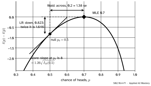
Draw the coin’s log-likelihood, measured from its peak, and mark the null value \({p_0 = 0.5}\). If the null were true, the peak should be near it. There are three natural ways to measure “near”.
S02.10.4-F1
One curve, three measurements of how far the null is from the peak: across (Wald), down (likelihood ratio) and the slope at the null (score).
The Wald test walks across: how many standard errors separate the estimate from the null? The likelihood-ratio test looks down: how much worse does the null explain the data than the best value does? The score test stands at the null and feels the slope: if the curve is steep there, the peak must be some way off. On a perfect parabola all three would say the same thing.
Build it up
Step 1. Wald. From lesson S02.10.3, \({\hat\theta}\) is approximately normal with standard error \({1/\sqrt{J(\hat\theta)}}\). Under \({H_0 : \theta = \theta_0}\),
\[
W = \frac{\hat\theta - \theta_0}{\widehat{\mathrm{se}}}
\]
is approximately standard normal. For the coin, \({W = 0.2/0.145 = 1.38}\).
Step 2. Score. At the null the score has mean 0 and variance \({I_n(\theta_0)}\) (lesson S02.10.1), and by the central limit theorem it is approximately normal. So
\[
S = \frac{U(\theta_0)}{\sqrt{I_n(\theta_0)}}
\]
is approximately standard normal. It needs no estimate at all, only the null. For the coin, \({U(0.5) = 7/0.5 - 3/0.5 = 8}\) and \({I_{10}(0.5) = 10/0.25 = 40}\), so \({S = 8/\sqrt{40} = 1.26}\).
Step 3. Likelihood ratio. Twice the drop from the peak to the null,
is never negative, and it is large when the null explains the data badly. For the coin, \({\ell(0.7) = -6.109}\) and \({\ell(0.5) = 10 \ln 0.5 = -6.931}\), so \({\Lambda = 2 \times 0.823 = 1.646}\).
Step 4. Why the factor 2. Near the peak, the curve is close to its parabola, \({\ell(\theta_0) \approx \ell(\hat\theta) - \tfrac12 J\,(\hat\theta - \theta_0)^2}\). Substituting,
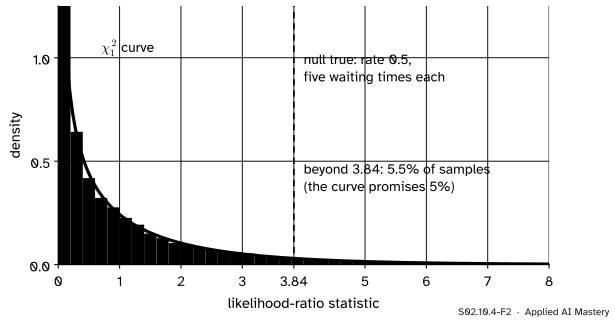
The square of a standard normal follows \({\chi^2_1}\) (S02.1.4), so \(\Lambda\) is compared with \({\chi^2_1}\). The approximation can be checked by simulation.
S02.10.4-F2
Wilks’s theorem tested on a small sample. With only five waiting times per sample, the likelihood-ratio statistic already follows \({\chi^2_1}\) closely: 5.5% of samples land beyond its 95% point, where the theory says 5%.
The formal statement
NoteThe three large-sample tests of \({H_0 : \theta = \theta_0}\)
Under \({H_0}\) and the regularity conditions of S02.10.3, \(W\) and \(S\) are approximately \({N(0, 1)}\), so \(W^2\) and \(S^2\) are approximately \({\chi^2_1}\). Wilks’s theorem (stated) says that \(\Lambda\) is approximately \({\chi^2_1}\) too. The two-sided p-values are \({2(1 - \Phi(\abs{W}))}\), \({2(1 - \Phi(\abs{S}))}\) and \({P(\chi^2_1 \ge \Lambda)}\).
All three are asymptotically equivalent: as \(n\) grows, the log-likelihood near its peak becomes a parabola, and on a parabola the across, down and slope measurements are one and the same. For small samples they differ, and none is exact.
Intervals by inversion. As in S02.5.4, a 95% interval is the set of null values a level-0.05 test does not reject. Each test gives its own:
Wald:\({\hat\theta \pm 1.96\,\widehat{\mathrm{se}}}\), symmetric by construction.
Score: every \({\theta_0}\) with \({\abs{S} \le 1.96}\). For a proportion this is the Wilson interval of S02.4.3.
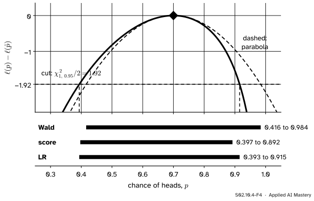
Likelihood ratio: every \({\theta_0}\) with \({\ell(\theta_0) \ge \ell(\hat\theta) - 1.92}\), where \({1.92 = \chi^2_{1,\,0.95}/2 = 3.841/2}\). Its ends solve an equation, found with a root finder.
S02.10.4-F4
Inverting the tests for 7 heads in 10. The likelihood-ratio interval is where the curve stays above the cut; the Wald interval is where the parabola does. The three intervals overlap heavily but are not the same.
Frontier note: where these three tests turn up in machine learning
Statistics packages print a Wald z for every logistic regression weight (S03.7). Comparing a model with a nested, smaller one is a likelihood-ratio test with as many degrees of freedom as the extra parameters, and the Akaike information criterion (M09.7) adds a penalty of 2 per parameter to the same \({-2\ell}\). The Laplace approximation of Bayesian inference (S04) replaces a posterior by the normal curve of S02.10.3, and the natural gradient (RL04.6) rescales a gradient by the inverse Fisher information matrix, so that steps are measured in the curvature of the likelihood.
Worked example
Test the coin, 7 heads in 10, against \({p_0 = 0.5}\) four ways, and give three 95% intervals.
S02.10.4-F3
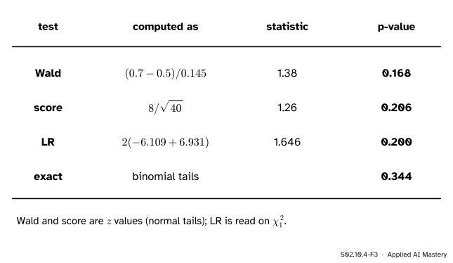
Three large-sample tests and the exact test on the same 10 tosses. None of the large-sample p-values reaches the exact 0.344, because 10 tosses are far from “large”.
Intervals. Wald \({0.7 \pm 1.96 \times 0.145}\), from 0.416 to 0.984; score (Wilson) 0.397 to 0.892; likelihood ratio 0.393 to 0.915. All three contain 0.5, matching “do not reject”.
The score and LR intervals lean to the left of 0.7, following the lopsided curve; the Wald interval cannot lean, and runs almost to 1.
Code
From scratch, with the normal tail from math.erf and the \({\chi^2_1}\) tail from the fact that \({P(\chi^2_1 \ge x) = P(\abs{Z} \ge \sqrt x)}\).
Wald 1.38 (p-value 0.168) score 1.26 (0.206) LR 1.646 (0.200)
The intervals: Wald by formula, score by Wilson’s formula, likelihood ratio by brentq, which needs a bracket on which the function changes sign. The function \({\ell(p) - \ell(\hat p) + 1.92}\) is positive at the peak and negative far from it.
from scipy import optimize, statsz, cut = stats.norm.ppf(0.975), stats.chi2.ppf(0.95, 1) /2wald = (p_hat - z * se, p_hat + z * se)centre = (p_hat + z**2/ (2* n)) / (1+ z**2/ n)half = z * math.sqrt(p_hat * (1- p_hat) / n + z**2/ (4* n**2)) / (1+ z**2/ n)score_ci = (centre - half, centre + half)f =lambda p: ell(p) - ell(p_hat) + cutlr_ci = (optimize.brentq(f, 1e-9, p_hat), optimize.brentq(f, p_hat, 1-1e-9))for name, ci in (("Wald", wald), ("score", score_ci), ("LR", lr_ci)):print(f"{name:5s}{ci[0]:.3f} to {ci[1]:.3f}")
Wald  0.416 to 0.984
score 0.397 to 0.892
LR    0.393 to 0.915
The same for the waiting times, against the exact interval from the fact that \({2\lambda \sum x_i}\) follows \({\chi^2_{2n}}\).
Wald [0.062 0.938] LR [0.179 1.075] exact [0.162 1.024]
The likelihood-ratio interval is much closer to the exact one than the Wald interval is. Last, the check of Wilks’s theorem behind the build-up figure (seed 5), and SciPy’s own tail areas.
Choose the coin or the waiting times, then raise the number of trials and watch the curve sharpen and the three interval bars close in on each other. Push the share of heads towards 0 or 1 to see the Wald interval run off the edge.
Pitfalls
S02.10.4-F5
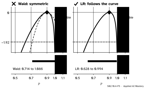
Wrong beside right. With 9 heads in 10 the curve is very lopsided. The Wald interval copies the parabola and claims values above 1; the likelihood-ratio interval follows the curve and stays inside.
“The three tests are interchangeable, so I can report whichever gives the smallest p-value.”
They agree only for large samples. For the coin they give 0.168, 0.206 and 0.200, and choosing after the fact is a forking path (S02.9). Decide in advance; when in doubt prefer the likelihood-ratio or score test, which look at the curve at the null value itself, over the Wald test, which judges the null by the curvature at the estimate.
“The Wald interval is always fine; it is what the software prints.”
Near the edge of the range it fails. With 9 heads in 10 it runs to 1.086; with 10 heads in 10 the estimated standard error is 0 and the interval is the single point 1. The likelihood-ratio interval for 10 in 10 is still sensible: it runs from \({e^{-1.92/10} = 0.825}\) to 1.
“Compare the likelihood-ratio statistic with 1.96.”
\(\Lambda\) is on the \({\chi^2_1}\) scale, whose 95% point is \({1.96^2 = 3.84}\). Its signed square root, \({\sqrt{1.646} = 1.28}\) with the sign of \({\hat\theta - \theta_0}\), is the one to compare with 1.96.
Check yourself
Recall
1. What does each of the three tests measure on the log-likelihood curve?
Show answer
Wald: the horizontal distance from the estimate to the null in standard errors. Score: the slope at the null, scaled by \({\sqrt{I_n(\theta_0)}}\). Likelihood ratio: twice the vertical drop from the peak to the null.
2. What does Wilks’s theorem say?
Show answer
Under the null and regularity conditions, \({\Lambda = 2(\ell(\hat\theta) - \ell(\theta_0))}\) is approximately \({\chi^2_1}\) for large \(n\) (one degree of freedom for one tested parameter).
3. Why do the three tests agree when the log-likelihood is a parabola?
Show answer
On \({\ell(\theta) = \ell(\hat\theta) - \tfrac12 J(\theta - \hat\theta)^2}\), the drop gives \({\Lambda = J(\hat\theta - \theta_0)^2 = W^2}\), and the slope at the null is \({J(\hat\theta - \theta_0)}\), so \({S = W}\) when \({I_n(\theta_0) = J}\).
4. Give the three 95% intervals for 7 heads in 10.
Show answer
Wald 0.416 to 0.984, score (Wilson) 0.397 to 0.892, likelihood ratio 0.393 to 0.915.
5. How is the likelihood-ratio interval defined, and how is it computed?
Show answer
It is the set of \(\theta\) with \({\ell(\theta) \ge \ell(\hat\theta) - 1.92}\). Its ends are the two roots of \({\ell(\theta) - \ell(\hat\theta) + 1.92 = 0}\), found with a bracketing root finder such as scipy.optimize.brentq.
Exercises
1.★ Test whether the waiting times (rate estimate 0.5, standard error 0.224) come from a rate of 1, with the Wald and likelihood-ratio tests.
so \({\Lambda = 2 \times 1.534 = 3.07}\), p-value \({P(\chi^2_1 \ge 3.07) = 0.080}\). The Wald test rejects at 0.05 and the likelihood-ratio test does not, a sign that five waiting times are not “large”.
2.★★ A classifier gets 90 of 100 test examples right. Test \({p_0 = 0.85}\) with all three tests.
p-value 0.140. None rejects at 0.05. They differ because the score test measures the spread at 0.85 and the Wald test at 0.9.
3.★★★ Show that for an exponential sample the score statistic for the rate equals the Wald statistic, so the two intervals coincide.
Show solution
With \({\ell(\lambda) = n\ln\lambda - \lambda\sum x_i}\), the score is \({U(\lambda_0) = n/\lambda_0 - n\bar x}\) and \({I_n(\lambda_0) = n/\lambda_0^2}\). So
For Wald, \({\hat\lambda = 1/\bar x}\) and \({\widehat{\mathrm{se}} = \hat\lambda/\sqrt n}\), so \(W = {\sqrt n(\hat\lambda - \lambda_0)/\hat\lambda} = {\sqrt n(1 - \lambda_0\bar x)}\). The two are equal, and inverting either gives \({\hat\lambda(1 \pm 1.96/\sqrt n)}\): 0.062 to 0.938 for the waiting times.
Summary card
One log-likelihood, three tests: across, slope and down.
S02.10.4-F1
Wald, score and likelihood ratio.
Wald.\({W = (\hat\theta - \theta_0)/\widehat{\mathrm{se}}}\): 1.38 for the coin.
Intervals. Invert each; the LR interval is \({\ell \ge \ell(\hat\theta) - 1.92}\).
Sources and next steps
Sources. Each was opened and checked against this lesson on 15 November 2026.
Philippe Rigollet, Parametric hypothesis testing slides, MIT OpenCourseWare 18.650, Fall 2016. Slides 21 and 22 build Wald’s test from the asymptotic normality of the MLE and compare its statistic with a chi-square quantile; slides 23 and 24 define the likelihood-ratio statistic \({2(\ell_n(\hat\theta_n) - \ell_n(\hat\theta_n^c))}\) and state that under the null it tends to a chi-square distribution.
Charles J. Geyer, Stat 5421 Lecture Notes: Statistical Inference for the Binomial Distribution, University of Minnesota. Section 8 names the Wald, Wilks (likelihood-ratio) and Rao (score) procedures and says they are asymptotically equivalent; Sections 9.1 to 9.3 give the three binomial intervals, the score interval by Wilson’s formula and the likelihood interval as a level set of the log-likelihood found by root finding; Sections 10.4, 10.7 and 10.8 give the three tests one-tailed, and Sections 11.1, 11.4 and 11.5 give them two-tailed, as they are used here.
SciPy reference, scipy.stats.chi2 (methods sf and ppf, shape parameter df) and scipy.optimize.brentq, which requires \({f(a)}\) and \({f(b)}\) to have opposite signs.
Next. This closes course S02’s likelihood thread. Logistic regression in S03.7 prints these Wald statistics for its weights, and model selection by information criteria (M09.7) starts from the same \({-2\ell}\).