No unbiased estimator can have a variance below 1 / (n I(theta)). Prove the bound from one covariance and the limit on a correlation, see the coin’s share of heads and the sample mean reach it, and see why the uniform’s corrected maximum is allowed to beat it.
S02.10.2L2 Intermediate25 minIn review (what this means)
The maths and code on this page are checked by automated tests on every change, but an independent reader has not signed it off yet. Spot a mistake or a confusing step? Tell us.
State the Cramér-Rao lower bound for an unbiased estimator and the conditions it needs.
Prove the bound by showing that an unbiased estimator has covariance 1 with the score and applying the limit on a correlation.
Compute the efficiency of an unbiased estimator and show that the share of heads and the sample mean are efficient.
Explain why the bound fails for the uniform on [0, theta] and why it applies only to unbiased estimators.
The question
A classifier is scored on 100 test examples, and its accuracy is estimated by the share it gets right. Could a cleverer formula, using the same 100 results, give an unbiased estimate with a smaller standard error? Or is there a floor below which no unbiased method can go, so that the only way to more precision is more data, or data that carry more information per point?
From the last lesson
1. What is the Fisher information of one coin toss with chance \(p\), and of 10 tosses at \({p = 0.7}\)?
2. What are the mean and variance of the score at the true parameter?
Show answer
Mean 0, and variance \({I_n(\theta) = n\,I(\theta)}\), the Fisher information.
Intuition
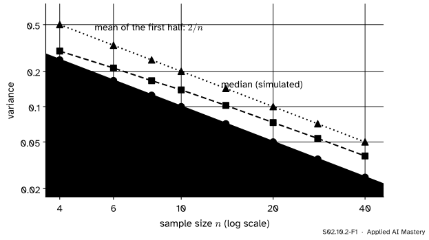
Take a normal population with standard deviation \({\sigma = 1}\) and estimate its mean from \(n\) draws. The sample mean, the median and the mean of only the first half of the data all aim at the right value, so all three are unbiased. Plot their variances against \(n\).
S02.10.2-F1
Three unbiased estimators of a normal mean. All of them shrink like \({1/n}\), but none ever enters the shaded region below \({\sigma^2/n}\). The sample mean lies on the floor itself.
Each estimator improves with more data, yet at every \(n\) the same line sits underneath them. That line is \({1/(n I(\mu))}\), one over the information in the sample. It is the Cramér-Rao lower bound, and the sample mean touches it: no unbiased estimator of a normal mean can do better.
Build it up
Step 1. Unbiased means “right on average, whatever the truth”. An estimator \(T\) is unbiased if \({\E_\theta[T] = \theta}\) for every value of \(\theta\) (S02.2.1). So if the truth moves up a little, the average of \(T\) must move up by exactly the same amount.
Step 2. The score says which way the data lean. From lesson S02.10.1, the score \(U(\theta)\) is positive when the sample looks like it came from a larger \(\theta\) and negative when it looks like a smaller one. An unbiased estimator has to follow those leanings, and the formal statement shows how strongly: its covariance with the score is exactly 1.
Step 3. A correlation cannot exceed 1. If \(T\) has covariance 1 with \(U\), then \(T\) must have enough spread to carry that covariance. The less \(T\) follows \(U\), the more spread it needs.
S02.10.2-F2
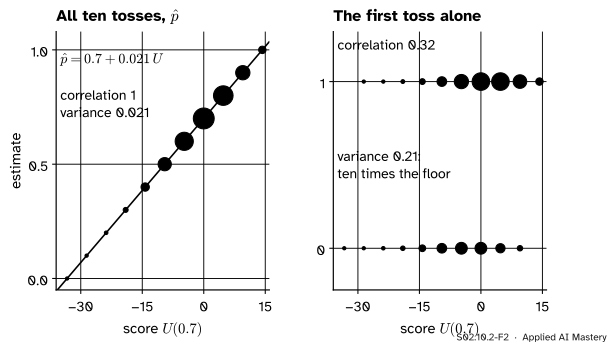
Left: the share of heads is an exact straight-line function of the score, correlation 1, and its variance is the floor. Right: the first toss alone is also unbiased, but it follows the score loosely, correlation 0.32, and pays with ten times the variance.
Step 4. Equality needs a straight line. A correlation equals 1 only when one variable is a straight-line function of the other. So the floor is reached exactly when \(T\) is a straight-line function of the score, as \({\hat{p}}\) is in the left panel.
The formal statement
NoteTheorem: the Cramér-Rao lower bound
Let \({X_1, \dots, X_n}\) be independent draws from \({f(x \mid \theta)}\), under the regularity conditions of S02.10.1 (in particular, the set of possible \(x\) does not depend on \(\theta\)). If \(T\) is an unbiased estimator of \(\theta\), then
Proof. Write \(\vect{x}\) for the whole sample and \({f_n(\vect{x} \mid \theta)}\) for its joint density, the product of the \(n\) single densities. Unbiasedness says, for every \(\theta\),
As in S02.10.1, \({\partial f_n / \partial\theta = f_n \cdot \partial \ln f_n/\partial\theta}\), and \({\partial \ln f_n / \partial\theta}\) is the score \(U\) of the whole sample. So
Dividing by \({n\,I(\theta)}\) gives the bound. \(\blacksquare\)
Efficiency. The efficiency of an unbiased estimator is the bound divided by its variance, a number between 0 and 1. An estimator with efficiency 1 is efficient. Equality in the correlation step needs \(T\) to be a straight-line function of \(U\), and since the slope must give covariance 1, the only candidate is
\[
T = \theta + \frac{U(\theta)}{n\,I(\theta)} .
\]
If this expression does not depend on the unknown \(\theta\), it is an efficient estimator. If it does, no unbiased estimator reaches the bound at that sample size.
Coin.\({p + \dfrac{k - np}{p(1-p)} \cdot \dfrac{p(1-p)}{n} = \dfrac{k}{n}}\): the share of heads is efficient.
Normal mean, \(\sigma\) known.\({I(\mu) = 1/\sigma^2}\), the bound is \({\sigma^2/n}\), and \({\operatorname{Var}(\bar x) = \sigma^2/n}\).
Exponential mean.\({I(\mu) = 1/\mu^2}\) (exercise 3 of S02.10.1), the bound is \({\mu^2/n}\), and \({\operatorname{Var}(\bar x) = \mu^2/n}\).
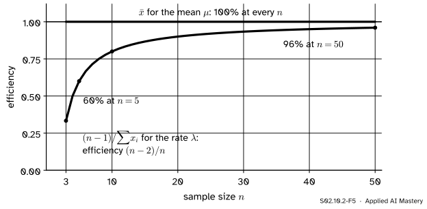
The exponential rate is different. For \({\lambda}\) the candidate is \({\lambda + \lambda^2(n/\lambda - \textstyle\sum x_i)/n = 2\lambda - \lambda^2 \bar x}\), which involves \(\lambda\). So no unbiased estimator of the rate is efficient. The unbiased \({(n - 1)/\sum x_i}\) has variance \({\lambda^2/(n - 2)}\) against the bound \({\lambda^2/n}\).
S02.10.2-F5
The same exponential data, two parameters. The sample mean is efficient for the mean at every \(n\); the best unbiased rate estimator only approaches the bound as \(n\) grows.
Go deeper: the variance of (n - 1) / sum of x
The sum \({S = \sum x_i}\) of \(n\) exponential waiting times has a gamma density \({\lambda^n s^{n-1} e^{-\lambda s}/(n - 1)!}\). For \({r < n}\),
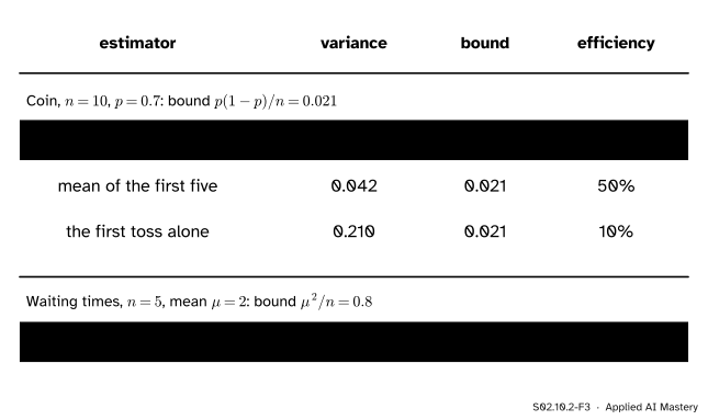
Compare four unbiased estimators with their bounds.
S02.10.2-F3
Each estimator’s variance against the Cramér-Rao bound. The efficiency says what share of the data an estimator effectively uses: half for the first five tosses, a tenth for the first toss.
The bound for the coin.\({I(0.7) = 1/0.21}\), so with \({n = 10}\) the bound is \({0.21/10 = 0.021}\).
All ten tosses.\({\operatorname{Var}(\hat p) = p(1-p)/n = 0.021}\): efficiency 100%.
The first five. Unbiased, with variance \({0.21/5 = 0.042}\): efficiency \({0.021/0.042 = 50\%}\). Throwing away half the tosses costs half the information.
The first toss. Unbiased, since \({\E[X_1] = p}\), with variance \({0.21}\): efficiency 10%. Its correlation with the score is \({\sqrt{0.1} = 0.32}\), as in the build-up figure.
The waiting times. With mean \({\mu = 2}\) and \({n = 5}\), the bound is \({\mu^2/n = 4/5 = 0.8}\), and \({\operatorname{Var}(\bar x) = \operatorname{Var}(X)/n = 4/5 = 0.8}\): efficient.
Code
From scratch: simulate 20,000 samples (seed 2) and measure the variance of each estimator.
import mathimport numpy as nprng = np.random.default_rng(2)tosses = rng.random((20_000, 10)) <0.7# True is a headv_all = tosses.mean(axis=1).var()v_five = tosses[:, :5].mean(axis=1).var()v_first = tosses[:, 0].var()print("bound 0.021 | all ten:", round(v_all, 4), " first five:", round(v_five, 4), " first toss:", round(v_first, 4))waits = rng.exponential(2.0, size=(20_000, 5)) # mean 2, rate 0.5print("bound 0.8 | sample mean:", round(waits.mean(axis=1).var(), 3))
bound 0.021 | all ten: 0.0211  first five: 0.0421  first toss: 0.2109
bound 0.8   | sample mean: 0.817
The simulated variances match the table to within the noise of 20,000 draws. Now the correlation of the first toss with the score, exactly: \({\operatorname{Cov} = 1}\), \({\operatorname{Var}(X_1) = 0.21}\) and \({\operatorname{Var}(U) = 47.6}\).
corr_first =1/ math.sqrt(0.21* (10/0.21))print("correlation of the first toss with the score:", round(corr_first, 3))
correlation of the first toss with the score: 0.316
The uniform on \({[0, \theta]}\) with \({\theta = 1}\) and \({n = 4}\), as many draws as the German tank serial numbers of S02.2.4: the corrected maximum \({\tfrac{5}{4}\max}\) against the would-be bound \({\theta^2/n = 0.25}\).
mean: 0.998 variance: 0.0419 theory 1/24 = 0.0417 'bound' 0.25
Finally SciPy: exact variances from the distributions, and the variance of the unbiased rate estimator \({4/S}\) from the gamma distribution of the sum (shape 5, scale 2), against the bound \({0.5^2/5 = 0.05}\).
The interactive of this module, curvature and intervals, lives in lesson S02.10.4. There, the sharper the curve, the narrower every interval, which is the Cramér-Rao bound seen from the other side.
Pitfalls
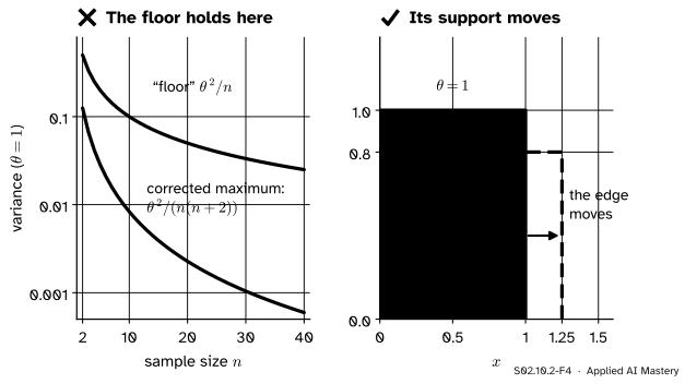
S02.10.2-F4
Wrong beside right. For the uniform on \({[0, \theta]}\) the corrected maximum has a variance far below \({\theta^2/n}\). Nothing is broken: the bound does not apply, because the edge of the data moves with \(\theta\).
“The Cramér-Rao bound holds for every model.”
The proof differentiated \({\int f\,dx = 1}\) under the integral sign, and that needs the range of possible \(x\) to stay put. For the uniform on \({[0, \theta]}\) the range ends at \(\theta\), and moving \(\theta\) moves the end. The would-be score \({-1/\theta}\) does not even average zero. The corrected maximum (the continuous version of the one in S02.2.4) has variance \({\theta^2/(n(n + 2))}\): for \({n = 4}\) that is \({\theta^2/24}\), six times below the “bound” \({\theta^2/4}\).
“No estimator can have a smaller error than the bound.”
Only unbiased ones. The estimator that always says \({\theta = 3}\) has variance 0. More usefully, the shrunken mean of S02.2.3 trades a little bias for less variance and can have a smaller mean squared error than any unbiased estimator. Ridge regression lives on that trade.
“An efficient estimator always exists.”
The bound is a floor, not a promise. The exponential rate has no unbiased estimator on the floor at any finite \(n\); the best has efficiency \({(n - 2)/n}\). Lesson S02.10.3 shows that the MLE reaches the floor in the limit of large \(n\), which is the sense in which it is called efficient.
Check yourself
Recall
1. State the Cramér-Rao lower bound.
Show answer
For an unbiased estimator \(T\) of \(\theta\) from \(n\) independent observations, under regularity conditions, \({\operatorname{Var}_\theta(T) \ge 1/(n\,I(\theta))}\).
2. What is the covariance of an unbiased estimator with the score, and what inequality turns it into the bound?
Show answer
It is 1. The bound on a correlation, \({\operatorname{Cov}(T, U)^2 \le \operatorname{Var}(T)\operatorname{Var}(U)}\), with \({\operatorname{Var}(U) = n\,I(\theta)}\).
3. What is the efficiency of an unbiased estimator?
Show answer
The bound divided by its variance, \({1/(n\,I(\theta)\operatorname{Var}(T))}\); efficient means 1.
4. What is the bound for the coin’s chance of heads from 10 tosses at \({p = 0.7}\), and which estimator reaches it?
Show answer
\({p(1-p)/n = 0.021}\), reached by the share of heads \({\hat p = k/n}\).
5. Why does the bound not apply to the uniform on \({[0, \theta]}\)?
Show answer
Its support ends at \(\theta\), so it moves with \(\theta\). The step that differentiates \({\int f\,dx = 1}\) under the integral sign fails, and the score does not average zero.
Exercises
1.★ For \(n\) Poisson counts, use \({I(\lambda) = 1/\lambda}\) (exercise 1 of S02.10.1) to find the bound, and show that the sample mean reaches it.
Show solution
The bound is \({1/(n/\lambda) = \lambda/n}\). A Poisson count has variance \(\lambda\), so \({\operatorname{Var}(\bar x) = \lambda/n}\), and \({\E[\bar x] = \lambda}\). The sample mean is unbiased with variance equal to the bound: efficient.
2.★★ A classifier’s accuracy is near 0.9. What is the smallest standard deviation any unbiased estimate of the accuracy from 100 test examples can have? How many examples bring that floor down to 0.01?
Show solution
Each example is a toss with \({I(p) = 1/(p(1-p))}\). The bound on the variance is \({p(1 - p)/n = 0.09/100 = 0.0009}\), so the standard deviation is at least \({\sqrt{0.0009} = 0.03}\). For 0.01 we need \({0.09/n = 0.0001}\), so \({n = 900}\). No formula can beat this; only more examples (or a cleverer design of the test) can.
3.★★★ Use the formula \({T = \theta + U(\theta)/(n\,I(\theta))}\) to show that the sample mean is efficient for the exponential mean \(\mu\), using \({I(\mu) = 1/\mu^2}\).
Show solution
For one waiting time the score in \(\mu\) is \({(x - \mu)/\mu^2}\), so for the sample \({U(\mu) = \sum (x_i - \mu)/\mu^2}\), and \({n\,I(\mu) = n/\mu^2}\). Then
The unknown \(\mu\) has cancelled, so \(T\) is a statistic, and it is a straight-line function of the score with covariance 1. It reaches the bound: \({\operatorname{Var}(\bar x) = \mu^2/n}\).
Summary card
No unbiased estimator has a variance below one over the information.
S02.10.2-F1
The floor \({1/(n I)}\), and the mean on it.
Bound.\({\operatorname{Var}(T) \ge 1/(n\,I(\theta))}\) for unbiased \(T\).
Proof.\({\operatorname{Cov}(T, U) = 1}\), and a correlation is at most 1.
Efficient.\({\hat p}\) for a coin; \({\bar x}\) for a normal or exponential mean.
Not for. Biased estimators, or a support that moves with \(\theta\).
Sources and next steps
Sources. Each was opened and checked against this lesson on 15 November 2026.
Stanford STATS 200, Autumn 2016, Lecture 15: Fisher information and the Cramer-Rao bound. Theorem 15.4 states the bound \({\operatorname{Var}_\theta[T] \ge 1/(nI(\theta))}\) for an unbiased estimator; its proof shows \({\operatorname{Cov}_\theta[T, Z] = 1}\) by differentiating the unbiasedness identity and applies the bound on a correlation, as here. The same section defines relative efficiency and an efficient estimator.
Philippe Rigollet, Maximum likelihood estimation slides, MIT OpenCourseWare 18.650, Fall 2016. Slide 23 lists, among the conditions for the large-sample theory of the MLE, that the support of the distribution does not depend on \(\theta\), the condition the uniform breaks.