Normal samples: the chi-square and t distributions
For a normal population the sampling distributions are exact. Meet the chi-square distribution as a sum of squared normals, the distribution of the sample variance, and the t distribution that appears when s replaces σ, with heavier tails that need 2.776 instead of 1.96 at n = 5.
S02.1.4L2 Intermediate25 minIn review (what this means)
The maths and code on this page are checked by automated tests on every change, but an independent reader has not signed it off yet. Spot a mistake or a confusing step? Tell us.
Define the chi-square distribution with k degrees of freedom as a sum of k squared standard normals, with mean k and variance 2k.
State that (n − 1)s²/σ² follows a chi-square distribution with n − 1 degrees of freedom for a normal sample, and derive the case n = 2.
Derive that (x̄ − μ)/(s/√n) follows a t distribution with n − 1 degrees of freedom, from the definition of t.
Compare t and normal quantiles and tail areas with scipy.stats.t and scipy.stats.chi2, and explain the heavier tails.
The question
You train a model five times with five random seeds and want to say how far the mean of the five scores is from the model’s long-run average. You do not know the true spread \(\sigma\), so you use the spread \(s\) of the five scores in its place and quote “mean plus or minus 1.96 standard errors”. How often is that statement wrong? Not 5 percent of the time but about 12, and this lesson finds the number that should replace 1.96.
From the last lesson
1. What is the skewness of the mean of \(n\) i.i.d. draws, if one draw has skewness \(\gamma\)?
Show answer
\(\gamma / \sqrt{n}\).
2. Why does the sampling distribution of the maximum not become normal?
Show answer
It cannot exceed the largest value in the population, and it piles onto that value as \(n\) grows.
Intuition
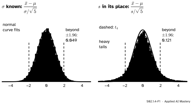
Take samples of five from a normal population with \(\mu = 10\) and \(\sigma = 2\). Standardise the mean in two ways: once with the true \(\sigma\), and once with each sample’s own \(s\) in its place.
S02.1.4-F1
The same 20,000 samples of five, standardised two ways. With \(\ctruth{\sigma}\) the statistic is normal (left). With \(s\) in its place it has heavier tails (right): 12 percent of it lies beyond \(\pm 1.96\). The dashed curve is the \(t\) distribution with 4 degrees of freedom.
Why should replacing \(\sigma\) by \(s\) matter? Because \(s\) is itself a statistic with a sampling distribution. In some samples it comes out much smaller than \(\sigma\), and then dividing by it inflates the statistic. Those samples make the long tails. This lesson finds the distribution of \(s^2\) (the chi-square) and then of the ratio (the \(t\)), exactly, when the population is normal.
Build it up
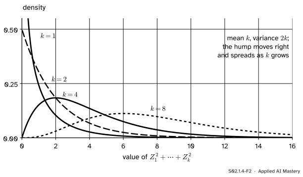
Step 1. Square and add normals. Let \(Z_1, \dots, Z_k\) be independent standard normals. The sum \(Z_1^2 + \cdots + Z_k^2\) has the chi-square distribution with \(k\) degrees of freedom, written \(\chi^2_k\). It is never negative. Its mean is \(k\), because each \(\E[Z_i^2] = {\operatorname{Var}(Z_i)} = 1\). Its variance is \(2k\): each \(Z_i^2\) has variance \({\E[Z_i^4] - 1} = {3 - 1} = 2\), using the normal’s kurtosis 3 (M06.7.4), and independent variances add.
S02.1.4-F2
Chi-square densities for \(k = 1, 2, 4\) and 8. Each is skewed to the right; as \(k\) grows the hump moves to the right, to the mean \(k\), and spreads.
Step 2. The sample variance is a scaled chi-square. For a sample of \(n\) from a normal population, \((n - 1)s^2/\sigma^2\) has the \(\chi^2_{n-1}\) distribution. It looks like a sum of \(n\) squared standardised deviations, \({\sum (x_i - \bar{x})^2/\sigma^2}\), but the deviations from \(\bar{x}\) always add to zero, so only \(n - 1\) of them are free. One degree of freedom is spent on estimating \(\mu\) by \(\bar{x}\).
Step 3. Divide a normal by a chi-square. Let \(Z\) be standard normal and \(V\) be \(\chi^2_\nu\), independent of \(Z\). The ratio
\[
T = \frac{Z}{\sqrt{V/\nu}}
\]
has the \(t\) distribution with \(\nu\) degrees of freedom, \(t_\nu\). The bottom line, \(V/\nu\), has mean 1, so \(T\) is a normal divided by something that is 1 on average but wobbles. The wobble fattens the tails, and less so as \(\nu\) grows and \(V/\nu\) settles at 1.
Step 4. The statistic we want is exactly such a ratio. The formal section shows that \((\bar{x} - \mu)/(s/\sqrt{n})\) is a \(t_{n-1}\) variable.
The formal statement
NoteTheorem (normal samples)
Let \(X_1, \dots, X_n\) be i.i.d. \(N(\mu, \sigma^2)\), with sample mean \(\bar{X}\) and sample variance \(S^2\) (divisor \({n - 1}\)). Then \(\bar{X}\) and \(S^2\) are independent,
The first two claims are stated here without a general proof. The case \(n = 2\) shows where they come from, and the third follows from them.
The case \(n = 2\), derived. With two values, \(\bar{X} = (X_1 + X_2)/2\), and the deviations are \({X_1 - \bar{X}} = {(X_1 - X_2)/2}\) and \({X_2 - \bar{X}} = {-(X_1 - X_2)/2}\). The divisor is \(n - 1 = 1\), so
The difference \(X_1 - X_2\) is normal with mean 0 and variance \(\sigma^2 + \sigma^2 = 2\sigma^2\), so \(Z = {(X_1 - X_2)/(\sigma\sqrt{2})}\) is standard normal, and
a \(\chi^2_1\) variable. Independence: \(\bar{X}\) depends on \(X_1 + X_2\) and \(S^2\) on \(X_1 - X_2\). These two are jointly normal, and their covariance is \({\operatorname{Var}(X_1) - \operatorname{Var}(X_2)} = 0\). For jointly normal variables, zero covariance means independence (M06.10.4), so \(\bar{X}\) and \(S^2\) are independent.
The \(t\) statistic, derived from the theorem. Divide top and bottom of the statistic by \(\sigma/\sqrt{n}\):
where \(Z = {(\bar{X} - \mu)/(\sigma/\sqrt{n})}\) is standard normal and \(V = (n - 1)S^2/\sigma^2\) is \(\chi^2_{n-1}\). The second line uses \({S/\sigma} = {\sqrt{S^2/\sigma^2}} = {\sqrt{V/(n-1)}}\). Since \(\bar{X}\) and \(S^2\) are independent, so are \(Z\) and \(V\), and Step 3 says the ratio is \(t_{n-1}\). The unknown \(\sigma\) has cancelled: the statistic can be computed from data and \(\mu\) alone.
S02.1.4-F5
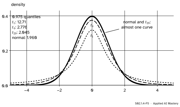
The \(t\) family. Fewer degrees of freedom mean a lower peak and fatter tails, so the point that cuts off the top 2.5 percent moves out, from 1.96 for the normal to 2.776 for \(t_4\) and 12.71 for \(t_1\).
The quantile that leaves 0.975 below it, \(t_{\nu, 0.975}\), and the chance of landing beyond \(\pm 1.96\):
\(\nu\)
\(t_{\nu, 0.975}\)
\(P(\abs{T} > 1.96)\)
1
12.706
0.300
4
2.776
0.122
9
2.262
0.082
29
2.045
0.060
99
1.984
0.053
normal
1.960
0.050
From about 30 degrees of freedom the \(t\) is hard to tell from the normal, but it is never the same.
Worked example
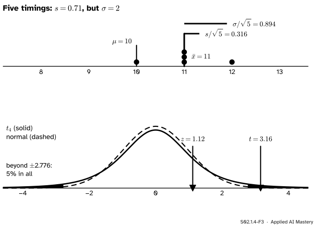
Five timings. A model’s inference time is normal with \(\mu = 10\) and \(\sigma = 2\) milliseconds (invented). Five timings come out 10, 11, 11, 12 and 11.
S02.1.4-F3
The same five timings standardised two ways. Their \(s\) is small by chance, so the yardstick \(s/\sqrt{5}\) is short, and the \(t\) statistic lands far out in the tail where \(z\) does not.
The mean and variance.\(\bar{x} = 55/5 = 11\). The deviations are \(-1, 0, 0, 1, 0\), whose squares add to 2, so \(s^2 = 2/4 = 0.5\) and \(s = 0.707\).
How unusual is that \(s\)? The chi-square statistic is \({(n - 1)s^2/\sigma^2} = {4 \times 0.5 / 4} = 0.5\). For \(\chi^2_4\) the chance of a value at most 0.5 is 0.026. So an \(s\) this small happens in only about one sample in forty.
Standardise with \(\sigma\).\(z = {(11 - 10)/(2/\sqrt{5})} = {1/0.894} = 1.118\). A value this far from 0 happens with chance 0.264 for a normal: not unusual.
Standardise with \(s\).\({s/\sqrt{5}} = {\sqrt{0.5/5}} = \sqrt{0.1} = 0.316\), so \(t = {1/0.316} = \sqrt{10} = 3.162\). That is beyond \(t_{4, 0.975} = 2.776\); for \(t_4\) the chance of a value at least this far from 0 is 0.034.
Read it. The mean is ordinary. The unusual thing is the small spread, and it made \(t\) large. The \(t_4\) distribution builds in exactly this risk, and that is why its tails are heavier than the normal’s.
Code
First the definitions, by simulation: a sum of three squared normals, and the \(z\) and \(t\) statistics of 20,000 normal samples of five.
import mathimport numpy as npfrom scipy import statsrng = np.random.default_rng(9)q = (rng.standard_normal((20_000, 3)) **2).sum(axis=1)print(f"chi-square 3 by simulation: mean {q.mean():.2f} (k = 3), variance {q.var():.2f} (2k = 6)")rng = np.random.default_rng(7)x = rng.normal(10, 2, size=(20_000, 5))xbar, s = x.mean(axis=1), x.std(axis=1, ddof=1)z = (xbar -10) / (2/ math.sqrt(5))t = (xbar -10) / (s / math.sqrt(5))v =4* s **2/2**2print(f"beyond 1.96: z {np.mean(np.abs(z) >1.96):.3f}, t {np.mean(np.abs(t) >1.96):.3f}; "f"t beyond 2.776: {np.mean(np.abs(t) >2.776):.3f}")print(f"(n-1)s^2/sigma^2: mean {v.mean():.2f} (4), variance {v.var():.2f} (8); "f"corr(x-bar, s^2) = {np.corrcoef(xbar, s **2)[0, 1]:.3f}")
chi-square 3 by simulation: mean 3.02 (k = 3), variance 6.06 (2k = 6)
beyond 1.96: z 0.049, t 0.121; t beyond 2.776: 0.050
(n-1)s^2/sigma^2: mean 3.98 (4), variance 7.91 (8); corr(x-bar, s^2) = -0.005
The simulated shares, 0.049, 0.121 and 0.050, match the exact values 0.05, 0.122 and 0.05 to within noise. Now the exact numbers from scipy.stats: ppf is the quantile function and sf the upper tail, \(1 - \text{cdf}\).
for nu in (1, 4, 9, 29, 99):print(f"nu = {nu:2d}: t quantile {stats.t.ppf(0.975, nu):.3f}, "f"P(|T| > 1.96) = {2* stats.t.sf(1.96, nu):.3f}")timings = np.array([10, 11, 11, 12, 11])s5 = timings.std(ddof=1)t5 = (timings.mean() -10) / (s5 / math.sqrt(5))print(f"s^2 = {s5 **2}, chi2 cdf at 0.5 = {stats.chi2.cdf(0.5, 4):.3f}, t = {t5:.3f}, "f"two-sided tail = {2* stats.t.sf(t5, 4):.3f}")
nu =  1: t quantile 12.706, P(|T| > 1.96) = 0.300
nu =  4: t quantile 2.776, P(|T| > 1.96) = 0.122
nu =  9: t quantile 2.262, P(|T| > 1.96) = 0.082
nu = 29: t quantile 2.045, P(|T| > 1.96) = 0.060
nu = 99: t quantile 1.984, P(|T| > 1.96) = 0.053
s^2 = 0.5000000000000001, chi2 cdf at 0.5 = 0.026, t = 3.162, two-sided tail = 0.034
Last, the same statistics for samples of five from the skewed city, where the theorem does not apply.
city: variance of (n-1)s^2/sigma^2 = 19.9 (8 if normal), corr(x-bar, s^2) = 0.70
city: t below -2.776: 0.128, above 2.776: 0.004
For the city the variance of \((n - 1)s^2/\sigma^2\) is about 19.9, not 8, and \(\bar{x}\) and \(s^2\) are strongly correlated (0.70): a sample that catches a Centre flat has both a high mean and a high spread. The \(t\) statistic then falls below \(-2.776\) in 12.8 percent of samples and above \(2.776\) in only 0.4 percent.
Explore
The module’s interactive, in lesson S02.1.3, draws samples from a skewed population. Set \(n = 5\) and the statistic to the mean: the read-out’s spread of the means matches \(\sigma/\sqrt{n}\), which uses the true \(\sigma\). This lesson is about what changes when you must estimate \(\sigma\) from each sample instead.
Pitfalls
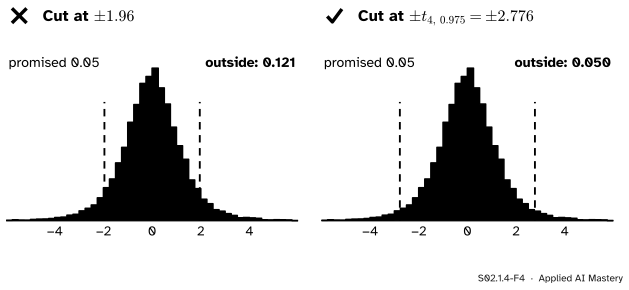
S02.1.4-F4
Wrong beside right. The same 20,000 \(t\) statistics from samples of five. Cut at \(\pm 1.96\), 12 percent fall outside. Cut at the \(t_4\) quantile \(\pm 2.776\), the promised 5 percent do.
“Plug in \(s\) for \(\sigma\) and keep using 1.96.”
With five runs of a model, “mean \(\pm\, 1.96\, s/\sqrt{5}\)” misses the long-run average 12 percent of the time instead of 5. Use \(t_{n-1, 0.975}\): 2.776 for five runs, 2.262 for ten. Lesson S02.4.2 builds the \(t\)-interval on this.
“The chi-square and \(t\) results hold for any population.”
They are exact only for a normal population. For samples of five from the skewed city the code above found the variance of \((n - 1)s^2/\sigma^2\) near 19.9 instead of 8, \(\bar{x}\) and \(s^2\) correlated at 0.70 instead of independent, and the \(t\) statistic lopsided: 12.8 percent below \(-2.776\) and 0.4 percent above. For large \(n\) the central limit theorem rescues the \(t\) statistic; for small \(n\) and skewed data it does not.
“A sample of \(n\) has \(n\) degrees of freedom.”
The variance \(s^2\) is built from deviations from \(\bar{x}\), which always add to zero, so one of them is fixed by the others. That leaves \(n - 1\) free deviations and \(\chi^2_{n-1}\), \(t_{n-1}\). With \(n = 5\), using \(t_5\) (quantile 2.571) instead of \(t_4\) (2.776) gives intervals that are too narrow.
Check yourself
Recall
1. How is the chi-square distribution with \(k\) degrees of freedom defined, and what are its mean and variance?
Show answer
As the distribution of \(Z_1^2 + \cdots + Z_k^2\) for independent standard normals; mean \(k\), variance \(2k\).
2. For a normal sample of size \(n\), what is the distribution of \((n - 1)s^2/\sigma^2\)?
Show answer
\(\chi^2_{n-1}\), and it is independent of \(\bar{x}\).
3. How is the \(t\) distribution with \(\nu\) degrees of freedom defined?
Show answer
As the distribution of \(Z/\sqrt{V/\nu}\) with \(Z\) standard normal and \(V \sim \chi^2_\nu\) independent of it.
4. What is \(t_{4, 0.975}\), and how often does a \(t_4\) variable fall beyond \(\pm 1.96\)?
Show answer
2.776; about 12 percent of the time (0.122).
5. Why does replacing \(\sigma\) by \(s\) make the tails heavier?
Show answer
Because \(s\) varies from sample to sample. When it comes out small, dividing by it makes the statistic large.
Exercises
1.★ Ten runs of a training script give scores with mean 0.812 and \(s = 0.010\). Find the multiplier that replaces 1.96, and how much wider than the normal one it makes the band \(\bar{x} \pm {\text{multiplier} \times s/\sqrt{n}}\).
Show solution
With \(n = 10\) there are \(\nu = 9\) degrees of freedom, so the multiplier is \(t_{9, 0.975} = 2.262\). The band is \(2.262/1.96 = 1.154\) times as wide, about 15 percent wider. Its half-width is \({2.262 \times 0.010 / \sqrt{10}} = 0.0072\).
2.★★ For a normal sample of five, how large must \(s^2/\sigma^2\) be before it is in the top 2.5 percent of its sampling distribution? Use \(\chi^2_{4, 0.975} = 11.14\).
Show solution
\(4 s^2/\sigma^2 \sim \chi^2_4\), so \({P(4 s^2/\sigma^2 > 11.14)} = 0.025\). Dividing by 4, \(s^2/\sigma^2 > 2.785\), which is \(s > 1.669\,\sigma\). So a sample of five has an \(s\) two-thirds larger than \(\sigma\) once in forty samples. Small samples estimate spread badly.
3.★★★ For \(n = 2\), show from the \(n = 2\) derivation that the \(t\) statistic is \(T = Z_1/\abs{Z_2}\) for two independent standard normals \(Z_1, Z_2\), and that this is the \(t_1\) of Step 3. How often does it fall beyond \(\pm 1.96\)?
Show solution
With \(n = 2\), \(S = \abs{X_1 - X_2}/\sqrt{2}\) and \(S/\sqrt{2} = \abs{X_1 - X_2}/2\). Put \(Z_1 = {(\bar{X} - \mu)/(\sigma/\sqrt{2})}\) and \(Z_2 = {(X_1 - X_2)/(\sigma\sqrt{2})}\). Both are standard normal, and they are independent because \({X_1 + X_2}\) and \({X_1 - X_2}\) are. Then
because \({\sigma\sqrt{2}/2} = {\sigma/\sqrt{2}}\). Since \(\abs{Z_2} = \sqrt{Z_2^2/1}\) with \(Z_2^2 \sim \chi^2_1\), this is Step 3 with \(\nu = 1\). It falls beyond \(\pm 1.96\) with probability 0.300, six times the normal’s 0.05, and its 0.975 quantile is 12.71.
Summary card
Estimating σ costs heavier tails: use t with n − 1 degrees of freedom.
S02.1.4-F1
\(\sigma\) known: normal. \(s\) in its place: \(t_{n-1}\).
Normal samples: \({(n - 1)s^2/\sigma^2} \sim \chi^2_{n-1}\), independent of \(\bar{x}\).
\(t_\nu = Z/\sqrt{V/\nu}\), so \({(\bar{x} - \mu)/(s/\sqrt{n})} \sim t_{n-1}\).
\(t_{4, 0.975} = 2.776\) against 1.96; stats.t.ppf, stats.chi2.ppf, .sf.
Sources and next steps
Sources. Each was opened and checked against this lesson on 15 November 2026.
Hossein Pishro-Nik, Introduction to Probability, Statistics, and Random Processes, Section 8.3.3: the chi-squared distribution as a sum of squared independent standard normals; the \(t\) distribution as \(Z/\sqrt{Y/n}\), whose density approaches the standard normal as \(n\) grows; Theorem 8.3 (\(\bar{X}\) and \(S^2\) independent, \({(n-1)S^2/\sigma^2} \sim {\chi^2(n-1)}\)) and Theorem 8.4 (\(T\) has a \(t\) distribution with \(n - 1\) degrees of freedom).
Jeremy Orloff and Jonathan Bloom, MIT OpenCourseWare 18.05, Reading 22: Confidence intervals based on normal data (Spring 2022). Section 5.2 builds \(t\) intervals by replacing \(\sigma\) with \(s\), with the studentized mean following \(t(n - 1)\); the section on chi-square intervals states that \((n - 1)s^2/\sigma^2\) follows a chi-square distribution with \(n - 1\) degrees of freedom.
David Diez, Mine Cetinkaya-Rundel and Christopher Barr, OpenIntro Statistics, 4th edition, Section 7.1.3: the \(t\) distribution has thicker tails than the normal, which is the correction needed for using \(s\) in place of \(\sigma\), and from about 30 degrees of freedom it is nearly indistinguishable from the normal.
SciPy reference, scipy.stats.t and scipy.stats.chi2: both take the degrees of freedom as df; ppf is the inverse of the cdf and sf is \(1 - \text{cdf}\).
Next. Module S02.2, Point estimation, asks what makes an estimator good and proves that \(s^2\) is unbiased for every \(n\); module S02.4 turns the \(t\) distribution into confidence intervals.