Put the new basis vectors in the columns of a matrix P. Multiplying by P turns new coordinates into standard ones, and multiplying by its inverse turns them back. Learn why, work both directions with numbers, and see why the direction feels backwards at first.
Build the change-of-basis matrix of a basis by writing its vectors as columns.
Convert coordinates from a new basis to the standard one by multiplying by P, and back by multiplying by the inverse of P.
Explain why P, although built from the new basis, converts new coordinates into old ones.
Predict how coordinates change when a basis vector is made longer.
In review. The maths and code on this page are checked by automated tests on every change, but an independent reader has not signed it off yet. Spot a mistake or a confusing step? Tell us.
The question
The last lesson found the new coordinates of one vector by solving two equations. A data set may hold a million vectors, and every one of them needs converting. Can the whole conversion be packed into a single matrix, and if so, which matrix converts back?
From the last lesson
1. What does \([\vect{v}]_B = (2, 1)\) say about the vector \(\vect{v}\)?
Show answer
That \(\vect{v} = 2\,\vect{b}_1 + 1\,\vect{b}_2\): the coordinates are the weights on the basis vectors of \(B\).
2. Which direction needs a system of equations: from new coordinates to the arrow, or from the arrow to new coordinates?
Show answer
From the arrow to its new coordinates. The other direction is just computing \(c_1\vect{b}_1 + c_2\vect{b}_2\).
Intuition
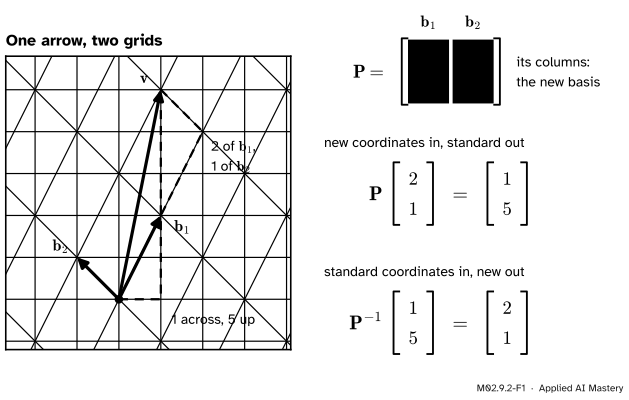
Think of two languages for naming arrows. The standard language counts steps of \(\ihat\) and \(\jhat\). The language of the basis \(B\) counts steps of \(\vect{b}_1 = (1, 2)\) and \(\vect{b}_2 = (-1, 1)\). An arrow is the same thing in both. Only its name differs.
Translating from\(B\) was the easy direction: compute \(c_1\vect{b}_1 + c_2\vect{b}_2\). But “weights times columns, added up” is exactly what a matrix does to a vector (lesson M02.4.2). So the translator is a matrix, and its columns are the new basis vectors.
M02.9.2-F1
The change-of-basis matrix\(\mat{P}\) has the new basis vectors as its columns. It turns new coordinates into standard coordinates, and its inverse turns them back.
This feels backwards at first. \(\mat{P}\) is built from the new basis, yet it converts out of the new coordinates, not into them. The reason is in its columns: they are the new basis vectors written in the standard language. \(\mat{P}\) knows what \(B\)’s words mean in our language, so it can translate \(B\)’s sentences into ours. Going the other way needs the inverse.
Build it up
Step 1. Rebuilding an arrow is a matrix product. With the basis vectors as columns,
Step 2. So \(\mat{P}\) takes new coordinates to standard ones. The left-hand side is the arrow \(\vect{v}\) itself, in standard coordinates. Hence \(\vect{v} = \mat{P}\,[\vect{v}]_B\).
Step 3. The inverse goes back.\(\mat{P}\) can be undone: a square matrix has an inverse exactly when it loses nothing (lesson M02.7.1 for the plane, lesson M02.7.4 for every size), and Step 3 of the formal section shows that a matrix whose columns are a basis loses nothing. Multiply both sides of \(\vect{v} = \mat{P}\,[\vect{v}]_B\) on the left by \(\mat{P}^{-1}\):
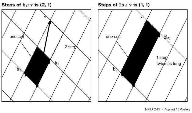
Step 4. Longer basis vectors mean smaller coordinates. This is why the inverse appears. If you measure a table in centimetres instead of metres, the unit shrinks by a factor of 100 and the number grows by a factor of 100. A basis vector is a unit of measurement. Make it longer and fewer copies are needed.
M02.9.2-F2
Double \(\vect{b}_1\) and the coordinate that counts it halves, from 2 to 1. The arrow has not changed. Basis vectors and coordinates always move in opposite directions.
Step 5. The columns of the inverse have a meaning too. Column 1 of \(\mat{P}^{-1}\) is \(\mat{P}^{-1}\ihat\), which by Step 3 is \([\ihat]_B\): the old basis vector \(\ihat\) written in the new language. So the two matrices mirror each other. \(\mat{P}\) holds the new basis in old coordinates. \(\mat{P}^{-1}\) holds the old basis in new coordinates.
The formal statement
NoteDefinition and result: the change-of-basis matrix
Let \(B\) be a basis \(\vect{b}_1, \dots, \vect{b}_n\) of \(\R^n\). Its change-of-basis matrix is the \({n \times n}\) matrix whose columns are the basis vectors,
Proof.Step 1: the first formula. Let \([\vect{v}]_B = (c_1, \dots, c_n)\). By the definition of coordinates, \(\vect{v} = c_1\vect{b}_1 + \cdots + c_n\vect{b}_n\). A matrix times a vector is the combination of its columns with the entries of the vector as weights, so the right-hand side is \(\mat{P}\,[\vect{v}]_B\).
Step 2: every vector is an output of \(\mat{P}\). By Step 1, the vector \(\vect{v}\) is \(\mat{P}\) applied to \([\vect{v}]_B\), and every \(\vect{v}\) has coordinates because a basis spans.
Step 3: \(\mat{P}\) loses nothing. Suppose \(\mat{P}\vect{c} = \vect{0}\). Then \(c_1\vect{b}_1 + \cdots + c_n\vect{b}_n = \vect{0}\), and a basis is independent, so every \(c_i\) is zero. Only the zero vector is sent to zero. If two inputs had the same output, \(\mat{P}\vect{c} = \mat{P}\vect{d}\), then \(\mat{P}{(\vect{c} - \vect{d})} = \vect{0}\), so \(\vect{c} = \vect{d}\): different inputs give different outputs.
Step 4: the second formula. Steps 2 and 3 say that the square matrix \(\mat{P}\) reaches every vector and never merges two, which is when it can be undone (lesson M02.7.1 for the plane, lesson M02.7.4 for every size). So \(\mat{P}^{-1}\) exists. Multiplying \(\vect{v} = \mat{P}\,[\vect{v}]_B\) on the left by it gives \(\mat{P}^{-1}\vect{v} = [\vect{v}]_B\). \(\blacksquare\)
The inverse in the plane. Lesson M02.7.1 derived the inverse of a 2 by 2 matrix. With the letters of the last lesson, \(\vect{b}_1 = (p, r)\) and \(\vect{b}_2 = (q, s)\), it reads
\[
\begin{bmatrix} p & q \\ r & s \end{bmatrix}^{-1}
= \frac{1}{ps - qr}\begin{bmatrix} s & -q \\ -r & p \end{bmatrix},
\]
provided \({ps - qr} \neq 0\). Multiply it by \((x, y)\) and the two rows give \(\frac{sx - qy}{ps - qr}\) and \(\frac{py - rx}{ps - qr}\). Those are the two formulas the last lesson found by elimination. The inverse matrix is that elimination, done once and stored.
Go deeper: converting between two bases, neither of them standard
Let a second basis \(C\) have change-of-basis matrix \(\mat{Q}\). The same arrow satisfies both \(\vect{v} = \mat{P}\,[\vect{v}]_B\) and \(\vect{v} = \mat{Q}\,[\vect{v}]_C\). Setting them equal and multiplying on the left by \(\mat{Q}^{-1}\),
Read from the right: \(\mat{P}\) translates from \(B\) into the standard language, then \(\mat{Q}^{-1}\) translates from the standard language into \(C\). The standard basis is the go-between.
With numbers. Let \(C\) be \((1, 1), (-1, 1)\). Its matrix has \({ps - qr} = {1 \cdot 1} - {(-1) \cdot 1} = 2\), so
Applied to \([\vect{v}]_B = (2, 1)\) this gives \(\tfrac12(6, 4) = (3, 2)\). Check: \(3\,(1, 1) + 2\,(-1, 1) = (1, 5)\), the same arrow.
Worked example
The basis is \(\vect{b}_1 = (1, 2)\), \(\vect{b}_2 = (-1, 1)\). Translate \([\vect{v}]_B = (2, 1)\) into standard coordinates, and translate \(\vect{w} = (2, 1)\) into \(B\).
M02.9.2-F3
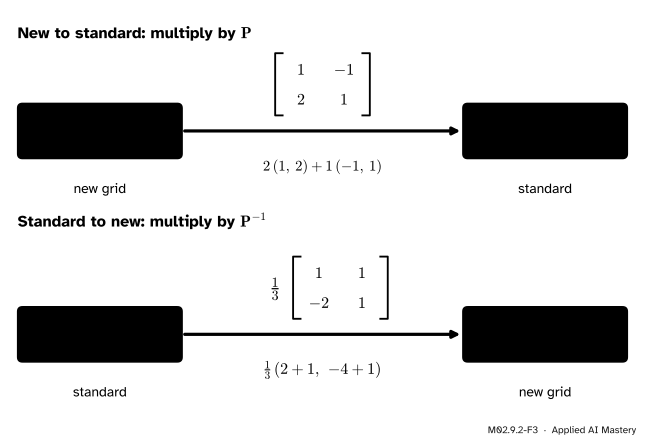
One vector translated each way. The matrix above each arrow does the translating, and the grey line under it is the arithmetic.
Build \(\mat{P}\). Write the basis vectors as columns: \(\mat{P} = \begin{bmatrix} 1 & -1 \\ 2 & 1 \end{bmatrix}\).
New to standard. Multiply by \(\mat{P}\), as a combination of its columns:
So \([\vect{w}]_B = (1, -1)\), the answer the last lesson reached by elimination.
Read the columns of \(\mat{P}^{-1}\). They are \((\tfrac13, -\tfrac23)\) and \((\tfrac13, \tfrac13)\), and they should be \(\ihat\) and \(\jhat\) in the new language. They are: \(\tfrac13(1, 2) - \tfrac23(-1, 1) = (1, 0)\) and \(\tfrac13(1, 2) + \tfrac13(-1, 1) = (0, 1)\).
Code
From scratch first: the product by columns and the 2 by 2 inverse formula.
def times(M, c):"""M times c as a combination of the columns of M (M is a list of rows).""" col1, col2 = (M[0][0], M[1][0]), (M[0][1], M[1][1])return (c[0] * col1[0] + c[1] * col2[0], c[0] * col1[1] + c[1] * col2[1])def inverse(M):"""The inverse of a 2 by 2 matrix [[p, q], [r, s]], from the formula.""" (p, q), (r, s) = M cell = p * s - q * rreturn [[s / cell, -q / cell], [-r / cell, p / cell]]P = [[1, -1], [2, 1]] # columns are b1 = (1, 2) and b2 = (-1, 1)P_inv = inverse(P)print("new (2, 1) -> standard", times(P, (2, 1)))print("standard (2, 1) -> new ", times(P_inv, (2, 1)))print("i-hat in the new language: ", times(P_inv, (1, 0)))print("j-hat in the new language: ", times(P_inv, (0, 1)))
new (2, 1)      -> standard (1, 5)
standard (2, 1) -> new      (1.0, -1.0)
i-hat in the new language:  (0.3333333333333333, -0.6666666666666666)
j-hat in the new language:  (0.3333333333333333, 0.3333333333333333)
Now NumPy, converting many vectors in one go. Each column of X is one vector.
import numpy as npP = np.array([[1.0, -1.0], [2.0, 1.0]])X = np.array([[1.0, 2.0, 4.0], [5.0, 1.0, 5.0]]) # columns: the vectors (1, 5), (2, 1), (4, 5)new = np.linalg.solve(P, X) # standard -> new, with no inverse formedprint("new coordinates, one column per vector:\n", new)print("translated back with P:\n", P @ new)print("the inverse, for reading:\n", np.linalg.inv(P))
new coordinates, one column per vector:
 [[ 2.  1.  3.]
 [ 1. -1. -1.]]
translated back with P:
 [[1. 2. 4.]
 [5. 1. 5.]]
the inverse, for reading:
 [[ 0.33333333  0.33333333]
 [-0.66666667  0.33333333]]
np.linalg.solve(P, X) gives \(\mat{P}^{-1}\mat{X}\) by elimination. It is the habit lesson M02.6.4 recommended: solve, and do not form the inverse unless you want to look at it.
Explore
M02.9-X1
Two-grid viewer
Drag the arrow \(\vect{v}\) or the tips of \(\vect{b}_1\) and \(\vect{b}_2\). The read-out gives both sets of coordinates, the matrix \(\mat{P}\) and its inverse. Every handle also has a slider, so the keyboard works too.
Things to try:
Leave the basis alone and move \(\vect{v}\) to \((2, 1)\). Do the new coordinates read \((1, -1)\), as in the worked example?
Press Standard basis. Why do the two sets of coordinates now agree, and what is \(\mat{P}\)?
Press Module basis, then Double b1. Which coordinate changes, and by what factor?
Press Swap b1 and b2. What happens to the coordinates and to the columns of \(\mat{P}\)?
Turn \(\vect{b}_2\) until it lies along \(\vect{b}_1\). Watch the coordinates grow larger and larger as the grid cells flatten, and read what the viewer says when the two arrows line up.
Pitfalls
M02.9.2-F4
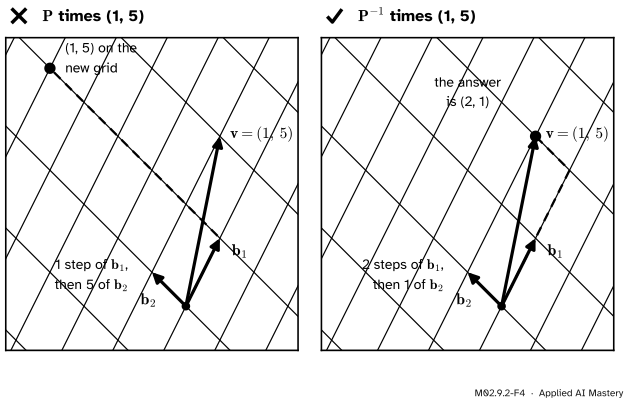
Wrong beside right. \(\mat{P}\) treats whatever it is given as steps on the new grid, so feeding it standard coordinates builds a different arrow. \(\mat{P}^{-1}\) answers the question that was asked.
“\(\mat{P}\) is built from the new basis, so \(\mat{P}\) converts into the new basis.”
It converts out of it. \(\mat{P}\,(1, 5)\) is \(1\,\vect{b}_1 + 5\,\vect{b}_2 = (-4, 7)\): the arrow that \(B\) would call \((1, 5)\), not the new name of our \((1, 5)\). To convert into the new basis use \(\mat{P}^{-1}\). A quick test: \(\mat{P}\) must send \((1, 0)\) to \(\vect{b}_1\), because \([\vect{b}_1]_B = (1, 0)\).
“Putting the basis vectors in the rows works just as well.”
That builds a different matrix, with rows \((1, 2)\) and \((-1, 1)\). It sends \((2, 1)\) to \({(1 \cdot 2 + 2 \cdot 1,\; -1 \cdot 2 + 1 \cdot 1)} = (4, -1)\), not to \((1, 5)\). Basis vectors go in the columns, because a matrix times a vector combines columns.
“Changing basis moves the vector.”
Nothing moves. The same arithmetic can be read two ways. Module M02.4 would read \(\mat{P}\) as a map that carries \(\ihat\) to \(\vect{b}_1\) and moves every arrow. Here it is a translator: the arrow stays and its name changes. Storing data in a better basis relies on the second reading. A compressed image keeps the coordinates \(\mat{P}^{-1}\vect{x}\) in a well-chosen basis, drops the small ones, and the viewer rebuilds a close copy of the picture with \(\mat{P}\).
Check yourself
Recall
1. How do you build the change-of-basis matrix of a basis?
Show answer
Write the basis vectors, in standard coordinates, as the columns of a matrix, in the order of the basis.
2. Which way does \(\mat{P}\) translate, and which way does \(\mat{P}^{-1}\) translate?
Show answer
\(\mat{P}\) takes new coordinates to standard ones, \(\vect{v} = \mat{P}\,[\vect{v}]_B\). Its inverse takes standard coordinates to new ones, \([\vect{v}]_B = \mat{P}^{-1}\vect{v}\).
3. Why is a change-of-basis matrix always invertible?
Show answer
Its columns are a basis. They span, so it reaches every vector. They are independent, so only the zero vector is sent to zero and no two inputs are merged. A map like that can be undone.
4. If you make a basis vector three times as long, what happens to the coordinate that counts it?
Show answer
It becomes a third of what it was. Basis vectors and coordinates change in opposite directions.
5. What do the columns of \(\mat{P}^{-1}\) hold?
Show answer
The standard basis vectors written in the new coordinates: column 1 is \([\ihat]_B\) and column 2 is \([\jhat]_B\).
Exercises
1.★ With this lesson’s \(\mat{P}\), translate \([\vect{x}]_B = (3, -1)\) into standard coordinates, and translate the standard vector \((0, 3)\) into \(B\).
2.★★ A basis \(C\) is made of \((2, 1)\) and \((1, 1)\). Write its change-of-basis matrix \(\mat{Q}\), find \(\mat{Q}^{-1}\), and find the coordinates of \((3, 2)\) in \(C\). Check your answer.
3.★★★ A basis \(\vect{b}_1, \vect{b}_2\) has change-of-basis matrix \(\mat{P}\). A second basis is \(k_1\vect{b}_1, k_2\vect{b}_2\) with \(k_1, k_2\) not zero. Show that the coordinates of any vector in the second basis are \({(c_1/k_1,\; c_2/k_2)}\), where \((c_1, c_2)\) are its coordinates in the first.
Show solution
Let \(\mat{K} = \begin{bmatrix} k_1 & 0 \\ 0 & k_2 \end{bmatrix}\). The columns of a product \(\mat{P}\mat{K}\) are \(\mat{P}\) applied to the columns of \(\mat{K}\) (lesson M02.5.2). Those are \(\mat{P}\,(k_1, 0) = k_1\vect{b}_1\) and \(\mat{P}\,(0, k_2) = k_2\vect{b}_2\), so the second basis has change-of-basis matrix \(\mat{P}\mat{K}\).
The inverse of a product reverses the order (lesson M02.7.1): \((\mat{P}\mat{K})^{-1} = \mat{K}^{-1}\mat{P}^{-1}\), and \(\mat{K}^{-1} = \begin{bmatrix} 1/k_1 & 0 \\ 0 & 1/k_2 \end{bmatrix}\) because that matrix times \(\mat{K}\) is the identity. So the new coordinates of \(\vect{v}\) are
With \(k_1 = 2\), \(k_2 = 1\) and \((c_1, c_2) = (2, 1)\) this gives \((1, 1)\), as in the second figure.
Summary card
Basis vectors in the columns: \(\mat{P}\) translates out of the new basis, \(\mat{P}^{-1}\) into it.
M02.9.2-F1
New in, standard out. Inverse: back.
The matrix.\(\mat{P} = \begin{bmatrix} \vect{b}_1 & \vect{b}_2 \end{bmatrix}\), basis vectors as columns.
New to standard.\(\vect{v} = \mat{P}\,[\vect{v}]_B\).
Standard to new.\([\vect{v}]_B = \mat{P}^{-1}\vect{v}\).
Between two bases.\([\vect{v}]_C = \mat{Q}^{-1}\mat{P}\,[\vect{v}]_B\).
Opposite directions. Scale a basis vector by \(k\) and its coordinate is divided by \(k\).
Sources and next steps
Sources. Each was opened and checked against this lesson on 12 November 2026.
Dan Margalit and Joseph Rabinoff, Interactive Linear Algebra, Section 5.3, Similarity (open textbook, Georgia Tech). It states that if the columns of \(C\) form a basis \(B\), then \(C[\vect{x}]_B = \vect{x}\) and \(C^{-1}\vect{x} = [\vect{x}]_B\). Section 2.8 defines the coordinates.
Grant Sanderson, Change of basis, 3Blue1Brown, Linear Algebra, chapter 13. The matrix whose columns are the other person’s basis vectors translates her language into ours, and its inverse translates ours into hers. The lesson stresses that this direction feels backwards.
Sheldon Axler, Linear Algebra Done Right, 4th edition (open access), Section 3D. Result 3.82 shows that the two matrices that convert between a pair of bases are inverses of each other, and example 3.83 works a 2 by 2 case.
Gilbert Strang, Change of basis; image compression, MIT OpenCourseWare 18.06SC, lecture 31. The lecture summary writes the rule as \(\vect{x} = \mat{W}\vect{c}\) and \(\vect{c} = \mat{W}^{-1}\vect{x}\), with the new basis in the columns of \(\mat{W}\), and uses it to store images compactly.
NumPy reference, numpy.linalg.solve and numpy.linalg.inv. solve accepts a matrix of right-hand sides, one per column, and inv returns the matrix whose product with the input is the identity.
Next.M02.9.3 The same map in a new basis uses \(\mat{P}\) and \(\mat{P}^{-1}\) together to rewrite a whole matrix, not just a vector, for a new basis.