Every matrix has four subspaces: the row space and null space among its inputs, the column space and left null space among its outputs. Derive the counting rule, rank plus nullity equals the number of columns, from pivots and free variables, and prove that the row space is perpendicular to the null space.
Name the four subspaces of an m-by-n matrix, say which space each lives in, and give its dimension in terms of the rank.
Derive the counting rule, rank plus nullity equals the number of columns, from pivot columns and free columns.
Prove that every vector of the row space is perpendicular to every vector of the null space.
Find bases of all four subspaces of a small matrix from one elimination.
Use the counting rule to show that a wide matrix always loses a direction and a tall matrix never fills its target.
In review. The maths and code on this page are checked by automated tests on every change, but an independent reader has not signed it off yet. Spot a mistake or a confusing step? Tell us.
The question
A layer takes 784 numbers in and gives 10 out. Without seeing a single weight you can say this: at least 774 independent directions of change in the input leave the output exactly as it was. Where does 774 come from? And where do those invisible directions sit, compared with the directions the layer does respond to?
From the last lesson
1. What is the null space of a matrix \(\mat{A}\)?
Show answer
The set of all inputs \(\vect{x}\) with \(\mat{A}\vect{x} = \vect{0}\). It is a subspace of the input space \(\R^n\).
2. If \(\vect{x}_p\) solves \(\mat{A}\vect{x} = \vect{b}\), what are all the solutions?
Show answer
\({\vect{x}_p + \vect{n}}\), where \(\vect{n}\) runs over the null space of \(\mat{A}\).
Intuition
We have met two subspaces: the column space, the outputs a matrix can reach, and the null space, the inputs it sends to zero. Each has a partner on its own side. Among the inputs, the partner of the null space is the row space, the span of the rows. Among the outputs, the partner of the column space is the left null space.
M02.7.4-F1
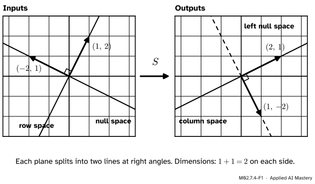
The four subspaces of the squash \(\mat{S} = \begin{bmatrix} 1 & 2 \\ 0.5 & 1 \end{bmatrix}\). On each side the two subspaces meet at a right angle, and their dimensions add up to 2.
The null space runs along \((-2, 1)\) (M02.7.3) and the column space along \((2, 1)\) (M02.7.2). The rows of \(\mat{S}\), \((1, 2)\) and \((0.5, 1)\), both lie along \((1, 2)\): that line is the row space. Two patterns are the subject of this lesson: the pairs are perpendicular, and the dimensions add up.
Build it up
Step 1. The rows live in the input space. A row of an \({m \times n}\) matrix has \(n\) entries, the same as an input. So the rows span a subspace of \(\R^n\), the row space. Write \(\mat{A}\T\), the transpose, for the matrix whose columns are the rows of \(\mat{A}\). Then the row space of \(\mat{A}\) is the column space of \(\mat{A}\T\).
Step 2. Why the right angle. By the row view of M02.4.2, entry \(i\) of \(\mat{A}\vect{x}\) is the dot product of row \(i\) with \(\vect{x}\). So \(\mat{A}\vect{x} = \vect{0}\) says that \(\vect{x}\) has dot product zero with every row. Dot product zero means perpendicular (M02.3.3). Check it on \(\mat{S}\) with \(\vect{x} = (-2, 1)\):
Step 3. The same on the output side. Apply Steps 1 and 2 to \(\mat{A}\T\). Its null space is perpendicular to its rows, and its rows are the columns of \(\mat{A}\). The null space of \(\mat{A}\T\) is the left null space of \(\mat{A}\): the vectors \(\vect{y}\) with \(\mat{A}\T\vect{y} = \vect{0}\). For \(\mat{S}\) it is the line along \(\vect{y} = (1, -2)\):
Read by columns, \(\mat{A}\T\vect{y}\) combines the rows of \(\mat{A}\) with weights \(y_1, \dots, y_m\). So a vector of the left null space is a recipe for combining the rows into the zero row: here, row 1 minus twice row 2.
Step 4. Count the columns. In the reduced form, every column either holds a pivot or is free. The pivot columns count the rank (M02.7.2). The free columns count the special solutions, which span the null space (M02.7.3). For the \({2 \times 3}\) matrix of the last lesson that reads \({2 + 1} = 3\). For the single row \(\begin{bmatrix} 1 & 2 & 0 \end{bmatrix}\) it reads \({1 + 2} = 3\).
M02.7.4-F2
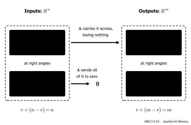
The big picture for any \({m \times n}\) matrix of rank \(r\). The inputs split into row space and null space, the outputs into column space and left null space.
The formal statement
NoteDefinition: the four subspaces
Let \(\mat{A}\) be an \({m \times n}\) matrix.
The column space: all combinations of the columns. A subspace of \(\R^m\).
The null space: all \(\vect{x}\) with \(\mat{A}\vect{x} = \vect{0}\). A subspace of \(\R^n\).
The row space: all combinations of the rows, which is the column space of \(\mat{A}\T\). A subspace of \(\R^n\).
The left null space: all \(\vect{y}\) with \(\mat{A}\T\vect{y} = \vect{0}\), which is the null space of \(\mat{A}\T\). A subspace of \(\R^m\).
Derivation. Let \(\mat{R}\) be the reduced form. It has \(r\) pivot columns, and \(r\) is the rank (M02.7.2). The other \({n - r}\) columns are free, so there are \({n - r}\) special solutions, and they span the null space (M02.7.3). They are also independent. Suppose \({c_1\vect{s}_1 + \dots + c_k\vect{s}_k} = \vect{0}\), and look at the entry in the position of the \(j\)-th free variable. There \(\vect{s}_j\) has a 1 and every other special solution has a 0, so that entry of the combination is \(c_j\), so \(c_j = 0\), for every \(j\). The special solutions are a basis of the null space, and the nullity is \({n - r}\). \(\blacksquare\)
In words: every input direction is either kept or lost.
The row space has dimension \(r\) too. Two facts give this.
Row operations do not change the row space. Each row of the new matrix is a combination of rows of the old one, so the new row space lies inside the old. Every row operation can be reversed by another row operation, so the old lies inside the new as well.
The non-zero rows of \(\mat{R}\) are a basis of it. They span the row space of \(\mat{R}\), since zero rows add nothing. They are independent by the argument just used: each has a 1 in its own pivot column, where the others have 0. There is one for each pivot, so there are \(r\) of them.
So a matrix and its transpose have the same rank: as many independent rows as independent columns.
The left null space has dimension \({m - r}\). Apply the counting rule to \(\mat{A}\T\), which has \(m\) columns and, as just shown, rank \(r\).
NoteResult: perpendicular pairs
Every vector of the row space is perpendicular to every vector of the null space. Every vector of the column space is perpendicular to every vector of the left null space.
Proof. Let \(\vect{x}\) be in the null space and let \(\vect{r}_1, \dots, \vect{r}_m\) be the rows. By Step 2, \({\vect{r}_i \cdot \vect{x}} = 0\) for each \(i\). A vector of the row space is a combination \(\vect{v} = {c_1\vect{r}_1 + \dots + c_m\vect{r}_m}\), and the dot product distributes over such a sum (M02.3.1):
The second statement is the first applied to \(\mat{A}\T\). \(\blacksquare\)
Three earlier promises can now be kept.
A wide matrix always loses something\({(n > m)}\). The rank is at most \(m\) (M02.7.2), so the nullity is \({n - r} \ge {n - m} > 0\). For the layer in the opening question, \({784 - 10} = 774\). A bias or an activation function changes nothing, since each acts only on the matrix’s output.
A tall matrix never fills its target\({(m > n)}\). The rank is at most \(n\), so the left null space has dimension \({m - r} \ge {m - n} > 0\). Take a non-zero \(\vect{y}\) in it. It is perpendicular to every output, but not to itself, since \({\vect{y} \cdot \vect{y}} = \norm{\vect{y}}^2 > 0\). So \(\vect{y}\) is not an output.
A square matrix that loses nothing reaches everything. If \(n = m\) and the null space is \(\{\vect{0}\}\), then \(r = n\), a pivot in every row, so no row reads “0 = something non-zero” (M02.7.2) and every target is reached.
Go deeper: a square matrix that loses nothing has an inverse
If an \({n \times n}\) matrix \(\mat{A}\) has null space \(\{\vect{0}\}\), it is invertible. By the counting rule the rank is \(n\): there are \(n\) pivots, one in every row and every column, so the reduced form is \(\mat{I}\). Elimination on \(\mat{A}\vect{x} = \vect{b}\) therefore ends with \(\mat{I}\vect{x}\) equal to a definite vector: exactly one solution, for every \(\vect{b}\). Let column \(j\) of a matrix \(\mat{B}\) be the solution of \(\mat{A}\vect{x} = \vect{e}_j\). Column by column this says \(\mat{A}\mat{B} = \mat{I}\). For the other product,
So each column of \({\mat{B}\mat{A} - \mat{I}}\) is sent to zero by \(\mat{A}\), and must be \(\vect{0}\). Hence \(\mat{B}\mat{A} = \mat{I}\) as well, and \(\mat{B} = \mat{A}^{-1}\).
For square matrices, one product is enough. Suppose \(\mat{B}\mat{A} = \mat{I}\). If \(\mat{A}\vect{x} = \vect{0}\), then \(\vect{x} = \mat{B}\mat{A}\vect{x} = \mat{B}\vect{0} = \vect{0}\). So the null space is \(\{\vect{0}\}\) and \(\mat{A}^{-1}\) exists. Then
so \(\mat{A}\mat{B} = \mat{I}\) too. Swapping the two names proves the converse.
Worked example
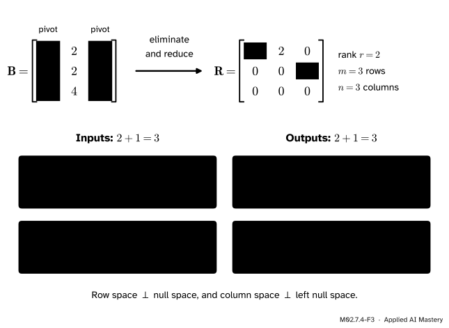
Find bases of all four subspaces of \(\mat{B} = \begin{bmatrix} 1 & 2 & 1 \\ 1 & 2 & 2 \\ 2 & 4 & 3 \end{bmatrix}\), and check the counting rule and the right angles.
M02.7.4-F3
One elimination, four bases: two from the reduced form \(\mat{R}\), one from the original matrix, and one from the record of the row operations.
Reduce. M02.7.2 did the work. The pivots are in columns 1 and 3, so \(r = 2\), with \(m = n = 3\).
Column space. Columns 1 and 3 of \(\mat{B}\) itself: \((1, 1, 2)\) and \((1, 2, 3)\). Dimension 2.
Row space. The non-zero rows of \(\mat{R}\): \((1, 2, 0)\) and \((0, 0, 1)\). Dimension 2.
Null space. The free variable is \(x_2\). The rows of \(\mat{R}\) say \({x_1 + 2x_2} = 0\) and \(x_3 = 0\), so the special solution is \((-2, 1, 0)\). Dimension \({3 - 2} = 1\).
Left null space. Its dimension is \({3 - 2} = 1\), so one vector is enough. Row 3 vanished when we formed
So row 1 plus row 2 minus row 3 is the zero row, and \(\vect{y} = (1, 1, -1)\). Check against each column of \(\mat{B}\): \({1 + 1 - 2} = 0\), then \({2 + 2 - 4} = 0\), then \({1 + 2 - 3} = 0\).
The left null space also explains M02.7.2, where a target could be reached exactly when \(b_3 = {b_1 + b_2}\). That condition is \({(1, 1, -1) \cdot \vect{b}} = 0\): the reachable targets are the ones perpendicular to the left null space.
Code
All four bases from one function, reusing rref from the last lesson.
The rref function from the last lesson
from fractions import Fractiondef rref(A):"""Reduced row echelon form. Returns it with the list of pivot columns (counted from 0).""" R = [[Fraction(x) for x in row] for row in A] rows, cols =len(R), len(R[0]) pivots, r = [], 0for c inrange(cols): usable = [i for i inrange(r, rows) if R[i][c] !=0]ifnot usable:continue R[r], R[usable[0]] = R[usable[0]], R[r] R[r] = [x / R[r][c] for x in R[r]]for i inrange(rows):if i != r: factor = R[i][c] R[i] = [x - factor * y for x, y inzip(R[i], R[r])] pivots.append(c) r +=1return R, pivots
def transpose(A):return [list(column) for column inzip(*A)]def special_solutions(A): R, pivots = rref(A) n, basis =len(R[0]), []for free in [c for c inrange(n) if c notin pivots]: s = [Fraction(0)] * n s[free] = Fraction(1)for row, p inzip(R, pivots): s[p] =-row[free] basis.append(s)return basisdef four_subspaces(A): R, pivots = rref(A)return {"column space": [[row[c] for row in A] for c in pivots], # pivot columns of A itself"row space": [row for row in R ifany(x !=0for x in row)], # non-zero rows of R"null space": special_solutions(A),"left null space": special_solutions(transpose(A)), }dot =lambda u, v: sum(a * b for a, b inzip(u, v))B = [[1, 2, 1], [1, 2, 2], [2, 4, 3]]spaces = four_subspaces(B)for name, basis in spaces.items():print(f"{name:>15}: dimension {len(basis)}, basis {[[int(x) for x in v] for v in basis]}")
The function returns \((-1, -1, 1)\) for the left null space: the worked example’s \((1, 1, -1)\) with the sign flipped, so the same line. Now test both results on random matrices, exactly.
import randomrandom.seed(0)for _ inrange(300): m, n, r = random.randint(1, 5), random.randint(1, 5), random.randint(0, 3) P = [[random.randint(-2, 2) for _ inrange(r)] for _ inrange(m)] Q = [[random.randint(-2, 2) for _ inrange(n)] for _ inrange(r)] A = [[sum(P[i][k] * Q[k][j] for k inrange(r)) for j inrange(n)] for i inrange(m)] # rank at most r s = four_subspaces(A) rank =len(s["column space"])assertlen(s["row space"]) == rank # row rank = column rankassert rank +len(s["null space"]) == n # the counting ruleassert rank +len(s["left null space"]) == m # the same rule for the transposeassertall(dot(u, v) ==0for u in s["row space"] for v in s["null space"])assertall(dot(u, v) ==0for u in s["column space"] for v in s["left null space"])print("counting rule and right angles hold on 300 random matrices")
counting rule and right angles hold on 300 random matrices
Last, the layer of the opening question.
import numpy as npfrom scipy.linalg import null_spacerng = np.random.default_rng(0)W = rng.normal(size=(10, 784)) # 784 numbers in, 10 outN = null_space(W) # its columns are a basis of the null spaceprint("rank:", np.linalg.matrix_rank(W), " nullity:", N.shape[1], " sum:", np.linalg.matrix_rank(W) + N.shape[1])print("largest entry of W @ N, to 12 places:", round(float(np.abs(W @ N).max()), 12))
rank: 10   nullity: 774   sum: 784
largest entry of W @ N, to 12 places: 0.0
The layer cannot see any of those 774 directions.
Explore
M02.7-X1
Subspace viewer
Left: the input space, with the null space in purple. Right: the output space, with the column space in vermillion. Drag the tips of the columns, or use the sliders, and watch the count change.
Things to try:
Press Squash onto a line and read the count: rank 1 plus nullity 1 makes 2 columns.
Press Step x along the null space a few times. The input \(\vect{x}\) moves. Does \(\mat{A}\vect{x}\)?
Press Show row space and left null space: four lines and two right angles, as in the anchor figure.
Drag the tip of \(\vect{a}_2\) off the line. What happens to the null space and the count?
Switch to 2 × 3 and press The matrix of M02.4.4. The null space is a line in space, along \((2, -1, 1)\). Try to make it disappear with the sliders. Why can you not?
Still in 2 × 3, press Rank 1. The null space is now a plane: \({1 + 2} = 3\).
Pitfalls
M02.7.4-F4
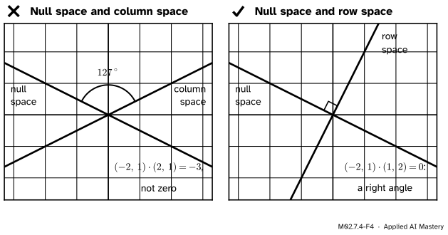
Wrong beside right, for the squash \(\mat{S}\). The null space is perpendicular to the row space, not to the column space.
“The null space is perpendicular to the column space.”
The perpendicular pairs sit on the same side: null space with row space among the inputs, column space with left null space among the outputs. For a matrix that is not square the two do not even live in the same space. For a square matrix the claim is usually false: for \(\mat{S}\), \({(-2, 1) \cdot (2, 1)} = -3\).
“Rank plus nullity equals the number of rows.”
It equals the number of columns: columns are what get sorted into pivot and free. A \({2 \times 3}\) matrix of rank 2 has nullity 1. The rows have their own count: rank plus the dimension of the left null space equals \(m\).
“The row space and the column space have the same dimension, so they are the same subspace.”
Same dimension, different sets. For \(\mat{S}\) the row space is the line along \((1, 2)\) and the column space is the line along \((2, 1)\). Only the number\(r\) is shared.
Check yourself
Recall
1. Name the four subspaces of an \({m \times n}\) matrix and say which space each lives in.
Show answer
Row space and null space, in the input space \(\R^n\). Column space and left null space, in the output space \(\R^m\).
2. Give the dimension of each in terms of \(m\), \(n\) and the rank \(r\).
Show answer
Row space \(r\), null space \({n - r}\), column space \(r\), left null space \({m - r}\).
3. State the counting rule.
Show answer
Rank plus nullity equals the number of columns: \({r + (n - r)} = n\).
4. Which pairs of subspaces are perpendicular?
Show answer
The row space and the null space. The column space and the left null space.
5. A \({3 \times 5}\) matrix has rank 2. What are the dimensions of its four subspaces?
Show answer
Row space 2, null space \({5 - 2} = 3\), column space 2, left null space \({3 - 2} = 1\).
Exercises
1.★ A matrix has 4 rows, 6 columns and rank 3. (a) Give the dimensions of its four subspaces. (b) Does \(\mat{A}\vect{x} = \vect{0}\) have non-zero solutions? (c) Can \(\mat{A}\vect{x} = \vect{b}\) be solved for every \(\vect{b}\)?
Show solution
(a) Row space 3, null space \({6 - 3} = 3\), column space 3, left null space \({4 - 3} = 1\).
(b) Yes: the null space has dimension 3.
(c) No. The left null space contains a non-zero \(\vect{y}\). Every output is perpendicular to \(\vect{y}\), and \(\vect{y}\) is not perpendicular to itself, so \(\vect{y}\) is never reached.
2.★★ Find bases of the four subspaces of \(\mat{A} = \begin{bmatrix} 1 & 2 & 0 \\ 0 & 1 & 1 \end{bmatrix}\), and check the two counts and the right angle.
Show solution
Subtracting twice row 2 from row 1 gives \(\mat{R} = \begin{bmatrix} 1 & 0 & -2 \\ 0 & 1 & 1 \end{bmatrix}\), with pivots in columns 1 and 2. So \(r = 2\), \(m = 2\), \(n = 3\).
Column space: columns 1 and 2 of \(\mat{A}\), \((1, 0)\) and \((2, 1)\). They span the whole plane. Row space: the rows of \(\mat{R}\), \((1, 0, -2)\) and \((0, 1, 1)\). Null space: the special solution \((2, -1, 1)\). Left null space: dimension \({m - r} = 0\), so it is \(\{\vect{0}\}\).
3.★★★ (a) Show that the only vector lying in both the row space and the null space of a matrix is \(\vect{0}\). (b) Deduce that if \(\vect{u}\) and \(\vect{v}\) are in the row space and \(\mat{A}\vect{u} = \mat{A}\vect{v}\), then \(\vect{u} = \vect{v}\).
Show solution
(a) Let \(\vect{v}\) be in both. Every vector of the row space is perpendicular to every vector of the null space, so \(\vect{v}\) is perpendicular to itself: \({\vect{v} \cdot \vect{v}} = 0\). But \({\vect{v} \cdot \vect{v}} = \norm{\vect{v}}^2\), and only the zero vector has length 0.
(b) By linearity \({\mat{A}(\vect{u} - \vect{v})} = {\mat{A}\vect{u} - \mat{A}\vect{v}} = \vect{0}\), so \({\vect{u} - \vect{v}}\) is in the null space. It is also in the row space, because the row space is a subspace. By (a), \({\vect{u} - \vect{v}} = \vect{0}\). This is the green arrow of the big picture: on its row space a matrix loses nothing.
Summary card
Every input direction is either kept or lost, and the kept ones are perpendicular to the lost ones.
Counting rule. Rank plus nullity equals the number of columns.
Wide\({(n > m)}\): the nullity is at least \({n - m}\). Tall\({(m > n)}\): some target is never reached.
Square. Null space \(\{\vect{0}\}\) exactly when the rank is \(n\), exactly when the matrix is invertible.
Sources and next steps
Sources. Each was opened and checked against this lesson on 12 November 2026.
Gilbert Strang, MIT OpenCourseWare 18.06SC, lecture summaries of The four fundamental subspaces and Orthogonal vectors and subspaces. The four subspaces, where each lies and its dimension; the row space of \(\mat{R}\) equals that of \(\mat{A}\); the row space is orthogonal to the null space, because \(\mat{A}\vect{x} = \vect{0}\) means dot product zero with each row.
Sheldon Axler, Linear Algebra Done Right, 4th edition (open access). The fundamental theorem of linear maps (3.21); a map to a lower-dimensional space is not injective (3.22) and one to a higher-dimensional space is not surjective (3.24); column rank equals row rank (3.57); for equal dimensions, injective, surjective and invertible are equivalent (3.65) and \(ST = I\) exactly when \(TS = I\) (3.68); and \(\text{null}\, T^* = (\text{range}\, T)^\perp\) (7.6).
Marc Deisenroth, Aldo Faisal and Cheng Soon Ong, Mathematics for Machine Learning. Section 2.6.2: a matrix and its transpose have equal rank. Theorem 2.24: rank-nullity.
Next. M02.8, Determinants as volume scaling, turns “is this square matrix invertible?” into a single number: the factor by which the map scales areas, which is zero exactly when something is lost.