The columns of a product AB are A applied to the columns of B. From that one fact, derive the row-times-column rule for every entry, multiply matrices by hand in two ways, write the three loops from scratch, and meet the @ operator.
State what the columns of a product AB are: A applied to each column of B.
Derive the row-times-column rule for the entries of a product from the column rule.
Multiply two small matrices by hand, column by column and entry by entry, and check that the two ways agree.
Write matrix multiplication from scratch with three loops, and use the @ operator in NumPy.
Explain why multiplying matching entries does not give the matrix of one map after another.
In review. The maths and code on this page are checked by automated tests on every change, but an independent reader has not signed it off yet. Spot a mistake or a confusing step? Tell us.
The question
Ask NumPy for A @ B and every entry of the answer is built from a whole row of one matrix and a whole column of the other. A neural network’s forward pass is mostly this one recipe, repeated. It looks arbitrary. Why not simply multiply the entries that sit in the same place? Where does the rule come from, and could you rebuild it if you forgot it?
From the last lesson
1. In the product \(\mat{A}\mat{B}\), which matrix acts first on a vector?
Show answer
\(\mat{B}\), the one on the right. \((\mat{A}\mat{B})\vect{v} = \mat{A}(\mat{B}\vect{v})\).
2. How do you find the matrix of “first \(\mat{B}\), then \(\mat{A}\)”?
Show answer
Follow \(\ihat\) and \(\jhat\) through both maps and write where they end up as columns. The columns are \(\mat{A}\vect{b}_1\) and \(\mat{A}\vect{b}_2\): \(\mat{A}\) applied to the columns of \(\mat{B}\).
Intuition
The last lesson defined the product \(\mat{A}\mat{B}\) as the matrix of “first \(\mat{B}\), then \(\mat{A}\)”, and found its columns by following the basis vectors. Look again at the journey of \(\ihat\). Its first stop was the first column of \(\mat{B}\). Its second stop was \(\mat{A}\) applied to that column. So:
Each column of \(\mat{A}\mat{B}\) is \(\mat{A}\) times the matching column of \(\mat{B}\).
That sentence is the whole of matrix multiplication. Everything else in this lesson is that sentence written out.
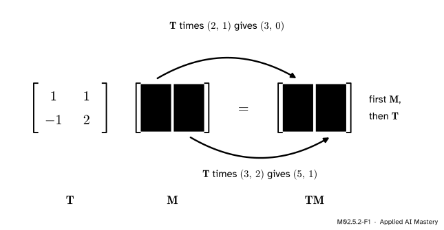
Try it with a friend from M02.4, the matrix \(\mat{T}\) of the map \(T(x, y) = (x + y,\; -x + 2y)\), and a second matrix \(\mat{M}\):
The product \(\mat{T}\mat{M}\), one column at a time. Each column of \(\mat{M}\) goes through \(\mat{T}\) on its own and comes out as the matching column of the product.
You have done both of these calculations before. M02.4.1 found \(T(2, 1) = (3, 0)\) and M02.4.2 found \(T(3, 2) = (5, 1)\). A product of two matrices is nothing new. It is several matrix-vector products, done side by side.
Build it up
Step 1. The columns of the product. The columns of \(\mat{M}\) are \((2, 1)\) and \((3, 2)\). Apply \(\mat{T}\) to each, by the column view of M02.4.2:
Put the two results side by side: \(\mat{T}\mat{M} = \begin{bmatrix} 3 & 5 \\ 0 & 1 \end{bmatrix}\).
Step 2. Open up the first column, one entry at a time. M02.4.2 gave a second way to compute a matrix-vector product, the row view: each entry of the answer is one row of the matrix times the vector. For the first column, \(\mat{T}\,(2, 1)\):
top entry: row 1 of \(\mat{T}\) is \((1, 1)\), and \(1 \cdot 2 + 1 \cdot 1 = 3\);
bottom entry: row 2 of \(\mat{T}\) is \((-1, 2)\), and \(-1 \cdot 2 + 2 \cdot 1 = 0\).
Step 3. The same for the second column,\(\mat{T}\,(3, 2)\):
top entry: \(1 \cdot 3 + 1 \cdot 2 = 5\);
bottom entry: \(-1 \cdot 3 + 2 \cdot 2 = 1\).
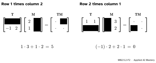
Step 4. See the pattern. Every entry of the product came from one row of the left matrix and one column of the right matrix. The entry in row \(i\) and column \(j\) used row \(i\) of \(\mat{T}\) and column \(j\) of \(\mat{M}\): multiply matching entries and add.
M02.5.2-F2
One entry of the product is one row of the left matrix times one column of the right matrix. The row number and the column number of the entry say which row and which column to use.
Step 5. Count the work. A \(2 \times 2\) product has 4 entries, and each needs 2 multiplications: 8 in all. For two \(n \times n\) matrices there are \(n^2\) entries with \(n\) multiplications each, which is \(n^3\). Doubling the size of the matrices makes the product eight times the work.
The formal statement
NoteDefinition: the product of two matrices
Let \(\mat{A}\) be an \(m \times n\) matrix and let \(\mat{B}\) be an \(n \times p\) matrix with columns \(\vect{b}_1, \dots, \vect{b}_p\). The product \(\mat{A}\mat{B}\) is the \(m \times p\) matrix whose columns are \(\mat{A}\) applied to the columns of \(\mat{B}\):
Each column \(\vect{b}_j\) has \(n\) entries, and \(\mat{A}\) accepts inputs with \(n\) entries (M02.4.4). That is why the number of columns of \(\mat{A}\) must equal the number of rows of \(\mat{B}\). In the plane all the numbers are 2. Lesson M02.5.4 looks at other shapes.
NoteResult 1: row times column
Write \(a_{ik}\) for the entry of \(\mat{A}\) in row \(i\) and column \(k\), and \(b_{kj}\) for the entry of \(\mat{B}\) in row \(k\) and column \(j\). The entry of \(\mat{A}\mat{B}\) in row \(i\) and column \(j\) is
It is row \(i\) of \(\mat{A}\) times column \(j\) of \(\mat{B}\).
Derivation. Column \(j\) of \(\mat{A}\mat{B}\) is the vector \(\mat{A}\vect{b}_j\), by the definition. The entry we want is entry \(i\) of that vector. The row view of M02.4.4 says that entry \(i\) of \(\mat{A}\vect{x}\) is \(a_{i1}x_1 + a_{i2}x_2 + \cdots + a_{in}x_n\). Put \(\vect{x} = \vect{b}_j\). The entries of \(\vect{b}_j\) are the entries of column \(j\) of \(\mat{B}\), namely \(x_1 = b_{1j},\; x_2 = b_{2j},\; \dots,\; x_n = b_{nj}\). Substituting them gives the formula.
The \(2 \times 2\) case, in letters. Let \(\mat{A} = \begin{bmatrix} a & b \\ c & d \end{bmatrix}\) and \(\mat{B} = \begin{bmatrix} e & f \\ g & h \end{bmatrix}\). The columns of \(\mat{B}\) are \((e, g)\) and \((f, h)\). Apply \(\mat{A}\) to each, by columns:
\[
\begin{aligned}
\mat{A}\begin{bmatrix} e \\ g \end{bmatrix}
&= e\begin{bmatrix} a \\ c \end{bmatrix} + g\begin{bmatrix} b \\ d \end{bmatrix} \\[0.4em]
&= \begin{bmatrix} ae + bg \\ ce + dg \end{bmatrix}, \\[0.8em]
\mat{A}\begin{bmatrix} f \\ h \end{bmatrix}
&= f\begin{bmatrix} a \\ c \end{bmatrix} + h\begin{bmatrix} b \\ d \end{bmatrix} \\[0.4em]
&= \begin{bmatrix} af + bh \\ cf + dh \end{bmatrix}.
\end{aligned}
\]
Side by side, these are the product:
\[
\begin{aligned}
&\begin{bmatrix} a & b \\ c & d \end{bmatrix}\begin{bmatrix} e & f \\ g & h \end{bmatrix} \\[0.4em]
&\quad= \begin{bmatrix} ae + bg & af + bh \\ ce + dg & cf + dh \end{bmatrix}.
\end{aligned}
\]
Check one entry against Result 1. The top right entry, \(af + bh\), is row 1 of \(\mat{A}\), which is \((a, b)\), times column 2 of \(\mat{B}\), which is \((f, h)\).
NoteResult 2: the product does both steps
For every vector \(\vect{x}\) with \(p\) entries, \((\mat{A}\mat{B})\,\vect{x} = \mat{A}\,(\mat{B}\vect{x})\).
The first line is the column view of \(\mat{B}\vect{x}\). The second holds because multiplying by \(\mat{A}\) is linear. The last line reads the definition of a matrix-vector product backwards: a combination of the columns \(\mat{A}\vect{b}_j\) of \(\mat{A}\mat{B}\), with the entries of \(\vect{x}\) as weights, is \((\mat{A}\mat{B})\vect{x}\).
Lesson M02.5.1 reached this result in the plane, by arguing that a linear map has only one matrix. Here it is a direct calculation, and it holds for every shape that fits.
Go deeper: the same two results with a summation sign
The index \(k\) walks along row \(i\) of \(\mat{A}\) and down column \(j\) of \(\mat{B}\) at the same time. Result 2 can then be proved entry by entry. Entry \(i\) of \((\mat{A}\mat{B})\vect{x}\) is
which is entry \(i\) of \(\mat{A}(\mat{B}\vect{x})\). The middle step swaps the order of two finite sums and takes \(a_{ik}\), which does not depend on \(j\), outside the inner sum. Both moves only regroup a finite list of terms.
Go deeper: a third way: row by row
The columns of \(\mat{A}\mat{B}\) are \(\mat{A}\) times the columns of \(\mat{B}\). There is a mirror image: row \(i\) of \(\mat{A}\mat{B}\) is row \(i\) of \(\mat{A}\) times \(\mat{B}\), a combination of the rows of \(\mat{B}\). For \(\mat{T}\mat{M}\), the top row is \(1\,(2, 3) + 1\,(1, 2) = (3, 5)\) and the bottom row is \(-1\,(2, 3) + 2\,(1, 2) = (0, 1)\). The reason is Result 1 read along a row: fix \(i\) and let \(j\) run. Strang’s lecture in the sources goes through these ways of seeing one product.
Worked example
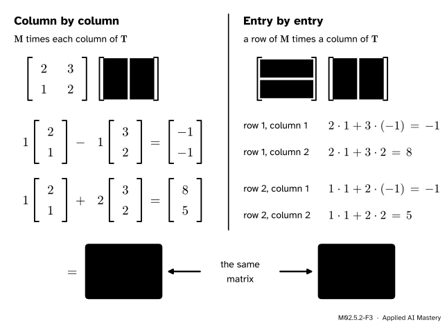
Multiply the same two matrices in the other order: find \(\mat{M}\mat{T}\), the matrix of “first \(\mat{T}\), then \(\mat{M}\)”, in both ways.
M02.5.2-F3
The product \(\mat{M}\mat{T}\) worked out twice. On the left, \(\mat{M}\) is applied to each column of \(\mat{T}\). On the right, each entry is a row of \(\mat{M}\) times a column of \(\mat{T}\).
Column by column. Now \(\mat{M}\) is on the left, so it is applied to the columns of \(\mat{T}\), which are \((1, -1)\) and \((1, 2)\). The columns of \(\mat{M}\) are \((2, 1)\) and \((3, 2)\).
Check with a vector. Take \(\vect{v} = (1, 1)\). In two steps, \(\mat{T}\vect{v} = (2, 1)\) and then \(\mat{M}\,(2, 1) = 2\,(2, 1) + 1\,(3, 2) = (7, 4)\). In one step, \((\mat{M}\mat{T})\vect{v} = (-1 + 8,\; -1 + 5) = (7, 4)\).
Compare. The build found \(\mat{T}\mat{M} = \begin{bmatrix} 3 & 5 \\ 0 & 1 \end{bmatrix}\). The same two matrices in the other order have given a different product. The next lesson is about that.
Code
From scratch, the entry rule is three loops: one over the rows of \(\mat{A}\), one over the columns of \(\mat{B}\), and one that walks along the row and down the column.
def matmul(A, B):"""A times B from scratch. A is m by n and B is n by p, each a list of rows.""" m, n, p =len(A), len(B), len(B[0])iflen(A[0]) != n:raiseValueError(f"A has {len(A[0])} columns but B has {n} rows") C = [[0] * p for _ inrange(m)]for i inrange(m): # each row of Afor j inrange(p): # each column of Bfor k inrange(n): # along the row, down the column C[i][j] += A[i][k] * B[k][j]return CT = [[1, 1], [-1, 2]]M = [[2, 3], [1, 2]]print("T M =", matmul(T, M))print("M T =", matmul(M, T))
T M = [[3, 5], [0, 1]]
M T = [[-1, 8], [-1, 5]]
The column rule is the same product, organised differently. It should give the same matrices, and the innermost line should run \(n^3\) times.
def matvec(A, x):"""A times x by columns (M02.4.4).""" result = [0] *len(A)for j inrange(len(x)):for i inrange(len(A)): result[i] += x[j] * A[i][j]return resultdef matmul_by_columns(A, B):"""Apply A to each column of B, then set the results side by side.""" p =len(B[0]) columns = [matvec(A, [row[j] for row in B]) for j inrange(p)]return [[columns[j][i] for j inrange(p)] for i inrange(len(A))]def count_multiplications(n):returnsum(1for i inrange(n) for j inrange(n) for k inrange(n))print("by columns:", matmul_by_columns(T, M), matmul_by_columns(M, T))print("multiplications for n = 2, 3, 100:", [count_multiplications(n) for n in (2, 3, 100)])
by columns: [[3, 5], [0, 1]] [[-1, 8], [-1, 5]]
multiplications for n = 2, 3, 100: [8, 27, 1000000]
In NumPy the product is the @ operator. It hands the work to compiled, highly optimised routines, so use it in place of your own loops. The Python loops above are far slower.
import numpy as npT, M = np.array([[1, 1], [-1, 2]]), np.array([[2, 3], [1, 2]])print("T @ M =", (T @ M).tolist(), " M @ T =", (M @ T).tolist())rng = np.random.default_rng(0)for _ inrange(200): A, B, x = rng.normal(size=(3, 4)), rng.normal(size=(4, 2)), rng.normal(size=2)assert np.allclose(A @ B, matmul(A.tolist(), B.tolist())) # the three loops agree with @assert np.allclose(A @ B, matmul_by_columns(A.tolist(), B.tolist()))assert np.allclose((A @ B) @ x, A @ (B @ x)) # Result 2print("200 random products: three loops = column rule = @, and (A @ B) @ x = A @ (B @ x)")
T @ M = [[3, 5], [0, 1]]   M @ T = [[-1, 8], [-1, 5]]
200 random products: three loops = column rule = @, and (A @ B) @ x = A @ (B @ x)
One near miss, which NumPy runs without complaint:
print("T * M =", (T * M).tolist(), " matching entries multiplied: not the product")
T * M = [[2, 3], [-1, 4]] matching entries multiplied: not the product
Explore
The composition explorer of this module is in lesson M02.5.3. It prints the product of the two matrices you choose. Pick the preset Shear and quarter turn, cover the product with your hand, and work out its four entries by row times column. Then check them against the read-out, and against the two arrows in the picture: they are the columns.
Pitfalls
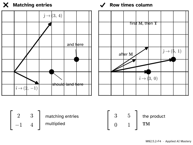
M02.5.2-F4
Wrong beside right. The rings mark where \(\ihat\) and \(\jhat\) really end up after \(\mat{M}\) and then \(\mat{T}\). The matrix made by multiplying matching entries sends them somewhere else.
“To multiply two matrices, multiply the entries that sit in the same place.”
That operation exists. It is called the entrywise or Hadamard product, it is what A * B does in NumPy, and it has its uses. But it is not the matrix of one map after another. For our matrices it gives \(\begin{bmatrix} 2 & 3 \\ -1 & 4 \end{bmatrix}\), which sends \(\ihat\) to \((2, -1)\). The real journey of \(\ihat\) is to \((2, 1)\) under \(\mat{M}\) and then to \((3, 0)\) under \(\mat{T}\). In machine-learning code, writing * where @ was meant is a classic bug, and when the shapes happen to allow it, nothing warns you.
“Row times column: any row with any column, from either matrix.”
The row comes from the left matrix and the column from the right one. Take them the other way round and you compute an entry of the other product. For row 1 and column 2: row 1 of \(\mat{T}\) times column 2 of \(\mat{M}\) is \(1 \cdot 3 + 1 \cdot 2 = 5\), an entry of \(\mat{T}\mat{M}\). Row 1 of \(\mat{M}\) times column 2 of \(\mat{T}\) is \(2 \cdot 1 + 3 \cdot 2 = 8\), an entry of \(\mat{M}\mat{T}\).
“The rule is a convention. Someone could have chosen a simpler one.”
The rule was not chosen. It was forced. Once you ask for the matrix that does “first \(\mat{B}\), then \(\mat{A}\)”, its columns must be \(\mat{A}\vect{b}_j\), and the row view turns that into row times column. Any other rule would give a matrix that does not describe the composition.
Check yourself
Recall
1. What are the columns of the product \(\mat{A}\mat{B}\)?
Show answer
\(\mat{A}\) applied to the columns of \(\mat{B}\): column \(j\) of \(\mat{A}\mat{B}\) is \(\mat{A}\vect{b}_j\).
2. How is the entry of \(\mat{A}\mat{B}\) in row \(i\) and column \(j\) computed?
Show answer
Take row \(i\) of \(\mat{A}\) and column \(j\) of \(\mat{B}\), multiply matching entries and add: \(a_{i1}b_{1j} + a_{i2}b_{2j} + \cdots + a_{in}b_{nj}\).
3. Write out the product of \(\begin{bmatrix} a & b \\ c & d \end{bmatrix}\) and \(\begin{bmatrix} e & f \\ g & h \end{bmatrix}\).
Show answer
\(\begin{bmatrix} ae + bg & af + bh \\ ce + dg & cf + dh \end{bmatrix}\).
4. How many multiplications does the entry rule use for two \(n \times n\) matrices, and why?
Show answer
\(n^3\): there are \(n^2\) entries, and each is a row times a column, which takes \(n\) multiplications.
5. In NumPy, what do A @ B and A * B compute?
Show answer
A @ B is the matrix product. A * B multiplies matching entries, which is a different operation.
Exercises
1.★ Compute \(\begin{bmatrix} 2 & -1 \\ 1 & 3 \end{bmatrix}\begin{bmatrix} 1 & 2 \\ 0 & 1 \end{bmatrix}\) column by column and entry by entry.
Show solution
Call the matrices \(\mat{A}\) and \(\mat{B}\). The columns of \(\mat{A}\) are \((2, 1)\) and \((-1, 3)\).
Both give \(\begin{bmatrix} 2 & 3 \\ 1 & 5 \end{bmatrix}\).
2.★★ Let \(\mat{D} = \begin{bmatrix} 2 & 0 \\ 0 & 3 \end{bmatrix}\) and \(\mat{A} = \begin{bmatrix} a & b \\ c & d \end{bmatrix}\). Compute \(\mat{D}\mat{A}\) and \(\mat{A}\mat{D}\). One of them scales the rows of \(\mat{A}\) and the other scales its columns. Which is which, and why?
\(\mat{D}\mat{A}\) scales the rows: row 1 by 2 and row 2 by 3. Reason: \(\mat{D}\) acts second, on the outputs of \(\mat{A}\), and it doubles every first coordinate and triples every second one. The first coordinates of the outputs are held in row 1 of \(\mat{A}\).
\(\mat{A}\mat{D}\) scales the columns: column 1 by 2 and column 2 by 3. Reason: \(\mat{D}\) acts first, sending \(\ihat\) to \(2\,\ihat\) and \(\jhat\) to \(3\,\jhat\). Then \(\mat{A}\) sends those to 2 times its first column and 3 times its second.
3.★★★ Use the entry rule to multiply two rotation matrices, \(\mat{R}(\alpha)\mat{R}(\beta)\), and show that the product is \(\mat{R}(\alpha + \beta)\). You may use the angle-addition formulas of M02.4.3.
Show solution
Write \(c_\alpha = \cos\alpha\), \(s_\alpha = \sin\alpha\), and the same for \(\beta\). The product is
The angle-addition formulas say \(\cos(\alpha + \beta) = c_\alpha c_\beta - s_\alpha s_\beta\) and \(\sin(\alpha + \beta) = s_\alpha c_\beta + c_\alpha s_\beta\). So the two entries on the diagonal are \(\cos(\alpha + \beta)\), the bottom left is \(\sin(\alpha + \beta)\) and the top right is \(-\sin(\alpha + \beta)\). The product is
Entry rule.\((\mat{A}\mat{B})_{ij} = a_{i1}b_{1j} + \cdots + a_{in}b_{nj}\): row \(i\) of \(\mat{A}\) times column \(j\) of \(\mat{B}\).
In the plane.\(\begin{bmatrix} a & b \\ c & d \end{bmatrix}\begin{bmatrix} e & f \\ g & h \end{bmatrix} = \begin{bmatrix} ae + bg & af + bh \\ ce + dg & cf + dh \end{bmatrix}\).
What it is for.\((\mat{A}\mat{B})\vect{x} = \mat{A}(\mat{B}\vect{x})\): the product does both steps.
In code.A @ B, not A * B. From scratch it is three loops and \(n^3\) multiplications.
Sources and next steps
Sources. Each was opened and checked against this lesson on 12 November 2026.
Sheldon Axler, Linear Algebra Done Right, 4th edition (open access). Section 3C chooses the definition of matrix multiplication (3.41) so that the matrix of a product of linear maps is the product of their matrices (3.43), as this lesson does. Result 3.46 is “entry of matrix product equals row times column” and result 3.48 is “column of matrix product equals matrix times column”.
Marc Deisenroth, Aldo Faisal and Cheng Soon Ong, Mathematics for Machine Learning, Cambridge University Press, 2020 (free PDF). Section 2.2.1, equation (2.13), gives the entry formula \(c_{ij} = \sum_l a_{il}b_{lj}\). A remark in the same section says that matrix multiplication is not an element-wise operation, and names the element-wise version the Hadamard product.
Gilbert Strang, Multiplication and inverse matrices, MIT OpenCourseWare 18.06SC. The lecture summary describes the product by row times column, by columns (“The product of matrix \(A\) and column \(j\) of matrix \(B\) equals column \(j\) of matrix \(C\)”), by rows, and by columns times rows.
NumPy manual, numpy.matmul. The @ operator is shorthand for np.matmul on arrays.
NumPy manual, Linear algebra. The introduction states that NumPy’s linear algebra functions rely on BLAS and LAPACK for efficient low-level implementations, and that @ is the preferred way to compute a matrix product of two-dimensional arrays.
Next.M02.5.3 Order matters asks which rules of ordinary multiplication survive, starting with the one that does not: \(\mat{T}\mat{M}\) and \(\mat{M}\mat{T}\) were different.