The projection of a vector onto a line is its shadow: the point of the line closest to it. Derive the formula by making the error perpendicular to the line, split any vector into a parallel and a perpendicular part, and see why this is the seed of least squares.
Compute the projection of one vector onto the line through another, and the error that is left over.
Derive the projection formula from the single condition that the error is orthogonal to the line.
Prove that the projection is the point of the line closest to the vector.
Split a vector into a part along a given direction and a part perpendicular to it.
Explain why the best slope of a line through the origin is a projection coefficient.
In review. The maths and code on this page are checked by automated tests on every change, but an independent reader has not signed it off yet. Spot a mistake or a confusing step? Tell us.
The question
You have a data point and a direction. You may keep only one number: how far to go along that direction. Which point of the line is closest to your data point, and what do you lose by moving there? Fitting a line to data and compressing data both ask this question, over and over.
From the last lesson
1. How do you test whether two vectors are orthogonal?
Show answer
Compute their dot product. They are orthogonal exactly when it is zero.
2. State the Cauchy-Schwarz inequality.
Show answer
\(\abs{\vect{a} \cdot \vect{b}} \le \norm{\vect{a}}\,\norm{\vect{b}}\), with equality exactly when one vector is a multiple of the other.
Intuition
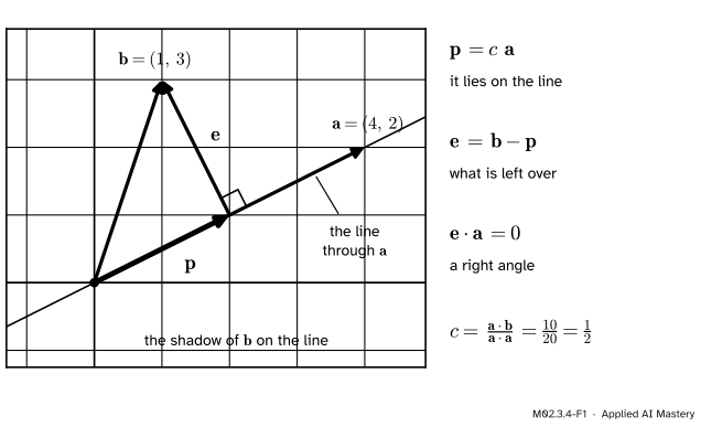
Draw the line through the origin in the direction of \(\vect{a}\). Now hold a lamp so that its light falls on the line at a right angle. The arrow \(\vect{b}\) casts a shadow on the line. That shadow is the projection of \(\vect{b}\) onto the line. We call it \(\vect{p}\).
M02.3.4-F1
The projection of \(\vect{b}\) onto the line through \(\vect{a}\). The shadow \(\vect{p}\) lies on the line, and the error \(\vect{e}\) that joins it to \(\vect{b}\) meets the line at a right angle.
What the shadow misses is the arrow from the tip of \(\vect{p}\) to the tip of \(\vect{b}\). That is \(\vect{e} = \vect{b} - \vect{p}\), the error. Two facts pin the shadow down:
\(\vect{p}\) lies on the line, and
\(\vect{e}\) is perpendicular to the line.
Those two facts are the whole lesson. They give a formula for \(\vect{p}\), and they make \(\vect{p}\) the point of the line closest to \(\vect{b}\).
Build it up
Step 1. One unknown number. Every point of the line is a multiple of \(\vect{a}\). So \(\vect{p} = c\,\vect{a}\) for some number \(c\), and finding the projection means finding \(c\).
Step 2. Every candidate has an error. Choose any \(c\). The point \(c\,\vect{a}\) misses \(\vect{b}\) by the arrow \(\vect{b} - c\,\vect{a}\).
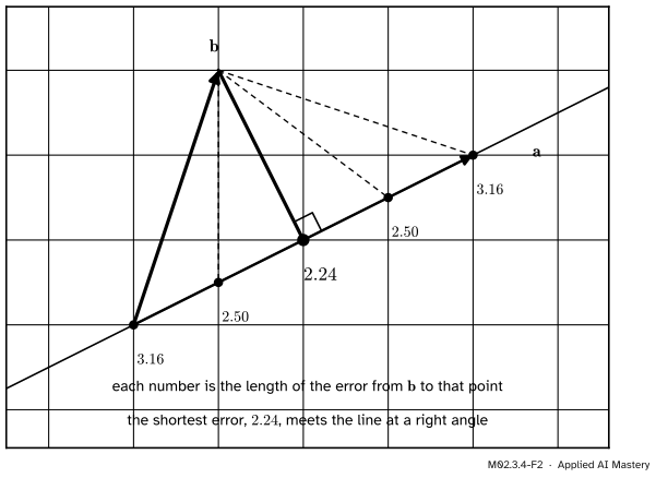
Step 3. Try a few. With the module’s pair \(\vect{a} = (4, 2)\) and \(\vect{b} = (1, 3)\), take \(c = 0, \tfrac14, \tfrac12, \tfrac34, 1\) and measure each error.
M02.3.4-F2
Five candidate points on the line and the length of the error from \(\vect{b}\) to each. The error is shortest at \(c = \tfrac12\), and that is the one that meets the line at a right angle.
The lengths fall and then rise again: \(3.16\), \(2.50\), \(2.24\), \(2.50\), \(3.16\). The shortest error belongs to \(c = \tfrac12\), and it is the only one that stands at a right angle to the line.
Step 4. Ask for the right angle. “Perpendicular” is a statement about a dot product, so it can be solved for \(c\). Require \(\vect{a} \cdot (\vect{b} - c\,\vect{a}) = 0\). The formal section does the algebra and gets \(c = \dfrac{\vect{a} \cdot \vect{b}}{\vect{a} \cdot \vect{a}}\). Here that is \(\tfrac{10}{20} = \tfrac12\), as the picture said.
Step 5. Split the vector. Now \(\vect{b} = \vect{p} + \vect{e}\): a part along \(\vect{a}\) plus a part perpendicular to \(\vect{a}\). Any vector can be split this way against any direction.
The formal statement
NoteDefinition: projection onto a line
Let \(\vect{a} \ne \vect{0}\) and \(\vect{b}\) be vectors in \(\R^n\). The projection of \(\vect{b}\) onto the line through \(\vect{a}\), and the error, are
The second line spreads the dot product over the difference and pulls out \(c\). The third divides by \(\vect{a} \cdot \vect{a} = \norm{\vect{a}}^2\), which is positive because \(\vect{a} \ne \vect{0}\). Exactly one \(c\) works, so there is exactly one projection.
Property 1: the error is orthogonal to the line. This is how \(c\) was chosen: \(\vect{a} \cdot \vect{e} = \vect{a} \cdot \vect{b} - c\,(\vect{a} \cdot \vect{a}) = \vect{a} \cdot \vect{b} - \vect{a} \cdot \vect{b} = 0\).
Property 2: the projection is the closest point. Take any other point \(t\,\vect{a}\) of the line. Split its error into the old error plus a step along the line:
The extra term is zero only when \(t = c\). So every other point of the line is strictly further from \(\vect{b}\) than \(\vect{p}\) is. The distance from \(\vect{b}\) to the line is \(\norm{\vect{e}}\).
Property 3: Pythagoras for the split.\(\vect{p}\) is a multiple of \(\vect{a}\), so it is orthogonal to \(\vect{e}\) too. Hence \(\norm{\vect{b}}^2 = \norm{\vect{p}}^2 + \norm{\vect{e}}^2\).
Property 4: only the line matters. Replace \(\vect{a}\) by \(k\vect{a}\) with \(k \ne 0\):
Doubling \(\vect{a}\) leaves the projection where it is. Doubling \(\vect{b}\) doubles it, because the 2 pulls out of \(\vect{a} \cdot (2\vect{b})\). With a unit vector \(\vect{u} = \vect{a} / \norm{\vect{a}}\) the bottom of the fraction is 1, and the formula becomes \(\vect{p} = (\vect{u} \cdot \vect{b})\,\vect{u}\).
Property 5: the length of the shadow. The number \(\vect{u} \cdot \vect{b} = \dfrac{\vect{a} \cdot \vect{b}}{\norm{\vect{a}}} = \norm{\vect{b}}\cos\theta\) is the scalar projection of \(\vect{b}\) on \(\vect{a}\): the length of the shadow, with a minus sign when the shadow points against \(\vect{a}\). Multiply it by \(\norm{\vect{a}}\) and you are back at the first lesson: the dot product is a length times a shadow.
Go deeper: projection as a map, and the matrix it will get
Fix the direction \(\vect{a}\) and let \(\vect{b}\) vary. The rules of the dot product give
So projecting a sum gives the sum of the projections, and projecting a multiple gives the multiple of the projection. A function with those two properties is a linear map, the subject of the next module, M02.4, and every linear map has a matrix. For \(\vect{a} = (4, 2)\) it is \(\begin{bmatrix} 0.8 & 0.4 \\ 0.4 & 0.2 \end{bmatrix}\): the first column is the projection of \((1, 0)\) and the second is the projection of \((0, 1)\).
Projecting twice changes nothing. \(\vect{p}\) is already on the line, and \(\dfrac{\vect{a} \cdot (c\,\vect{a})}{\vect{a} \cdot \vect{a}}\,\vect{a} = c\,\vect{a} = \vect{p}\).
Frontier note: from one line to least squares and PCA
Replace the line by a plane, or by a subspace of any dimension, and the same two facts still define the projection: it lies in the subspace, and the error is orthogonal to the subspace. Least-squares regression is that projection (M02.10). Principal component analysis asks the question the other way round: for a cloud of data points, which line makes the projections lose the least? Mathematics for Machine Learning introduces projections with exactly these two uses in mind (the opening of Section 3.8).
Worked example
Project \(\vect{b} = (1, 3)\) onto the line through \(\vect{a} = (4, 2)\).
M02.3.4-F3
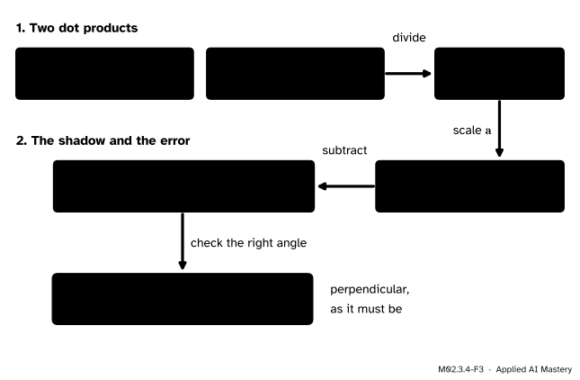
The trace of the calculation: two dot products, one division, one scaling, one subtraction and one check.
Check the right angle: \(\vect{e} \cdot \vect{a} = (-1)(4) + (2)(2) = 0\).
The lengths agree with property 3: \(\norm{\vect{p}}^2 + \norm{\vect{e}}^2 = 5 + 5 = 10 = \norm{\vect{b}}^2\). The distance from \(\vect{b}\) to the line is \(\norm{\vect{e}} = \sqrt{5} \approx 2.24\), the smallest number in the figure of Step 3.
A shadow that points backwards. Project \((-2, 1)\) onto the same line. \(c = \tfrac{-8 + 2}{20} = -0.3\), so \(\vect{p} = (-1.2, -0.6)\) and \(\vect{e} = (-0.8, 1.6)\). The angle is obtuse, so \(c\) is negative and the shadow lies on the far side of the origin. The check still works: \(\vect{e} \cdot \vect{a} = -3.2 + 3.2 = 0\).
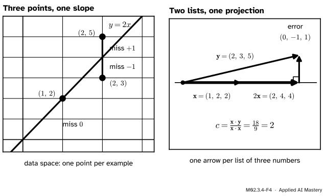
The seed of least squares. Three measurements \((x, y)\) are \((1, 2)\), \((2, 3)\) and \((2, 5)\). Which line through the origin, \(y = c\,x\), fits them best?
M02.3.4-F4
One fit, seen in two spaces. Left: each example is a point, and the line misses two of them. Right: all the \(x\)-values form one arrow and all the \(y\)-values another. The best slope is the projection coefficient, and the list of misses is the error arrow.
Collect the three \(x\)-values into one vector, \(\vect{x} = (1, 2, 2)\), and the three \(y\)-values into another, \(\vect{y} = (2, 3, 5)\). A slope \(c\) predicts the values \(c\,\vect{x}\), and its misses are the entries of \(\vect{y} - c\,\vect{x}\). “Best” usually means the smallest sum of squared misses, and that sum is \(\norm{\vect{y} - c\,\vect{x}}^2\). So we want the point of the line through \(\vect{x}\) that is closest to \(\vect{y}\). By property 2 that is the projection:
The fitted values are \(2\vect{x} = (2, 4, 4)\) and the misses are \(\vect{y} - 2\vect{x} = (0, -1, 1)\), with squared length 2. They are orthogonal to \(\vect{x}\): \(0 - 2 + 2 = 0\). A slope of \(1.9\) or \(2.1\) gives a sum of squares of \(2.09\), exactly the \(\norm{\vect{e}}^2 + (c - t)^2\,\norm{\vect{x}}^2 = 2 + 0.01 \cdot 9\) that property 2 predicts.
One caution about the two panels. The misses in the left panel are vertical, because each one compares two \(y\)-values of a single example. The right angle is not in that picture. It lives in the right panel, where a whole list of three numbers is one arrow.
Code
From scratch first.
import mathdef dot(a, b):returnsum(x * y for x, y inzip(a, b))def project(b, a):"""The projection of b onto the line through a, and the error that is left over."""if dot(a, a) ==0:raiseValueError("the zero vector does not give a line") c = dot(a, b) / dot(a, a) p = [c * x for x in a] e = [y - q for y, q inzip(b, p)]return c, p, ea, b = (4, 2), (1, 3)c, p, e = project(b, a)print("c =", c, " p =", p, " e =", e, " e . a =", dot(e, a))print("squared lengths: p", dot(p, p), " e", dot(e, e), " b", dot(b, b))for t in (0, 0.25, 0.5, 0.75, 1): miss = [y - t * x for x, y inzip(a, b)]print(" candidate", t, " error length", round(math.sqrt(dot(miss, miss)), 2))print("obtuse case:", [round(v, 2) for part in project((-2, 1), a)[1:] for v in part])
c = 0.5   p = [2.0, 1.0]   e = [-1.0, 2.0]   e . a = 0.0
squared lengths: p 5.0  e 5.0  b 10
  candidate 0  error length 3.16
  candidate 0.25  error length 2.5
  candidate 0.5  error length 2.24
  candidate 0.75  error length 2.5
  candidate 1  error length 3.16
obtuse case: [-1.2, -0.6, -0.8, 1.6]
With NumPy the formula is one line. The loop then tests the five properties on random vectors with five entries.
import numpy as npdef proj(b, a):return (a @ b) / (a @ a) * aa, b = np.array([4.0, 2.0]), np.array([1.0, 3.0])print("p =", proj(b, a), " with a doubled:", proj(b, 2* a), " with b doubled:", proj(2* b, a))u = a / np.linalg.norm(a)print("scalar projection u . b =", round(u @ b, 4), " and (u . b) u =", np.round((u @ b) * u, 10))rng = np.random.default_rng(0)for _ inrange(1000): a5, b5 = rng.normal(size=(2, 5)) p5 = proj(b5, a5) e5 = b5 - p5assertabs(e5 @ a5) <1e-9# property 1 t = rng.normal()assert np.linalg.norm(b5 - t * a5) >= np.linalg.norm(e5) -1e-12# property 2assert np.isclose(b5 @ b5, p5 @ p5 + e5 @ e5) # property 3assert np.allclose(proj(b5, -3.7* a5), p5) # property 4assert np.isclose(np.linalg.norm(p5), abs(a5 @ b5) / np.linalg.norm(a5)) # property 5assert np.allclose(proj(p5, a5), p5) # projecting twiceprint("the five properties hold on 1000 random pairs")
p = [2. 1.]   with a doubled: [2. 1.]   with b doubled: [4. 2.]
scalar projection u . b = 2.2361   and (u . b) u = [2. 1.]
the five properties hold on 1000 random pairs
The least-squares example, by projection and then with NumPy’s own solver.
x, y = np.array([1.0, 2.0, 2.0]), np.array([2.0, 3.0, 5.0])slope = (x @ y) / (x @ x)misses = y - slope * xprint("slope by projection:", slope, " misses:", misses, " misses . x =", misses @ x)print("sum of squares at 1.9, 2 and 2.1:", [round(float(np.sum((y - t * x) **2)), 2) for t in (1.9, 2.0, 2.1)])solution = np.linalg.lstsq(x.reshape(-1, 1), y, rcond=None)[0]print("slope from numpy.linalg.lstsq:", solution)
slope by projection: 2.0   misses: [ 0. -1.  1.]   misses . x = 0.0
sum of squares at 1.9, 2 and 2.1: [2.09, 2.0, 2.09]
slope from numpy.linalg.lstsq: [2.]
Explore
M02.3-X1
Projection explorer
Drag the tips of \(\vect{a}\) and \(\vect{b}\) and watch the shadow, the error and the right angle follow. The read-out gives the dot product, the angle, the cosine and the projection. Every handle also has a slider, so the keyboard works too.
Things to try:
Press Lesson example. Does the read-out give \(c = 0.50\), \(\vect{p} = (2, 1)\) and \(\vect{e} = (-1, 2)\), as in the worked example?
Move the slider Your guess away from the projection. The dashed line is the error of your guess. Can you make it shorter than the solid one?
Drag \(\vect{b}\) round the origin. Where is it when the dot product is zero? What happens to the shadow when the angle passes \(90^\circ\)?
Press Halve a. Which numbers in the read-out change, and which stay the same?
Stretch \(\vect{b}\) without turning it. Watch the dot product grow while the cosine stays put.
Pitfalls
M02.3.4-F5
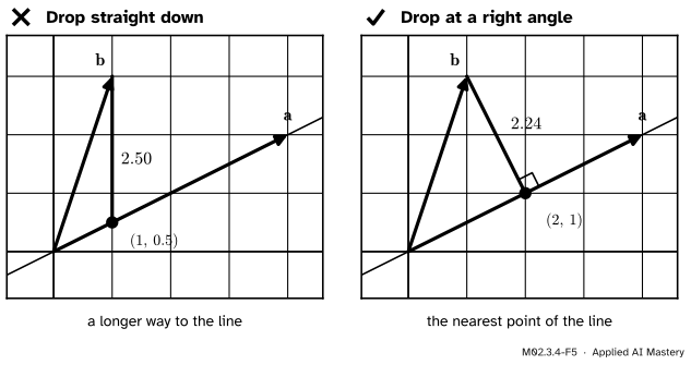
Wrong beside right. Straight down means at a right angle to the horizontal axis, which is the wrong line. The projection meets the line through \(\vect{a}\) at a right angle, and its path is shorter.
“To project, drop straight down onto the line.”
“Down” is perpendicular to the horizontal axis, not to the line you are projecting onto. From \(\vect{b} = (1, 3)\) the vertical drop reaches the line at \((1, 0.5)\), a distance of \(2.5\) away. The projection \((2, 1)\) is only \(2.24\) away. The right angle must be with the line through \(\vect{a}\).
“Divide by the length of \(\vect{a}\).”
The formula divides by \(\vect{a} \cdot \vect{a}\), the length squared. One factor of the length turns \(\vect{a} \cdot \vect{b}\) into the length of the shadow. The other turns \(\vect{a}\) into a unit vector to walk along. Dividing only once gives \(\tfrac{10}{\sqrt{20}}(4, 2) \approx (8.94, 4.47)\), far beyond the true \((2, 1)\). The two formulas agree only when \(\vect{a}\) is a unit vector.
“Projecting \(\vect{b}\) onto \(\vect{a}\) is the same as projecting \(\vect{a}\) onto \(\vect{b}\).”
The dot product does not care about order. The projection does. Projecting \(\vect{b} = (1, 3)\) onto \(\vect{a} = (4, 2)\) gives \((2, 1)\), a point of the line through \(\vect{a}\). Projecting \(\vect{a}\) onto \(\vect{b}\) gives \(\tfrac{10}{10}(1, 3) = (1, 3)\), a point of the line through \(\vect{b}\).
Check yourself
Recall
1. Write the formula for the projection of \(\vect{b}\) onto the line through \(\vect{a}\).
2. What is true of the error \(\vect{e} = \vect{b} - \vect{p}\)?
Show answer
It is orthogonal to the line: \(\vect{a} \cdot \vect{e} = 0\).
3. In what sense is the projection the best point of the line?
Show answer
It is the closest one to \(\vect{b}\): every other point of the line is further away.
4. What happens to the projection if \(\vect{a}\) is doubled? If \(\vect{b}\) is doubled?
Show answer
Doubling \(\vect{a}\) changes nothing, because only the line matters. Doubling \(\vect{b}\) doubles the projection.
5. What does the formula become when the direction is a unit vector \(\vect{u}\)?
Show answer
\(\vect{p} = (\vect{u} \cdot \vect{b})\,\vect{u}\): the scalar projection times the unit direction.
Exercises
1.★ Project \(\vect{b} = (3, 4)\) onto the line through \(\vect{a} = (2, 1)\). Find \(\vect{p}\) and \(\vect{e}\), and check that \(\vect{e}\) is orthogonal to \(\vect{a}\).
Show solution
\(\vect{a} \cdot \vect{b} = 6 + 4 = 10\) and \(\vect{a} \cdot \vect{a} = 4 + 1 = 5\), so \(c = 2\). Then \(\vect{p} = 2\,(2, 1) = (4, 2)\) and \(\vect{e} = (3, 4) - (4, 2) = (-1, 2)\). Check: \(\vect{e} \cdot \vect{a} = -2 + 2 = 0\). The shadow is twice as long as \(\vect{a}\): a projection can reach beyond the arrow that marks the line.
2.★★ Project the data vector \(\vect{b} = (1, 2, 3)\) onto the line through \(\vect{a} = (1, 1, 1)\). What do the entries of \(\vect{p}\) and of \(\vect{e}\) mean in terms of the three numbers 1, 2 and 3? How far is \(\vect{b}\) from the line?
Show solution
\(\vect{a} \cdot \vect{b} = 1 + 2 + 3 = 6\) and \(\vect{a} \cdot \vect{a} = 3\), so \(c = 2\) and \(\vect{p} = (2, 2, 2)\). The coefficient is the sum of the entries divided by how many there are: the mean. So \(\vect{p}\) holds the mean in every entry.
\(\vect{e} = (1, 2, 3) - (2, 2, 2) = (-1, 0, 1)\): each number minus the mean. Subtracting the mean from data, called centring, is removing its projection onto the all-ones vector. Check: \(\vect{e} \cdot \vect{a} = -1 + 0 + 1 = 0\), which says that deviations from the mean add up to zero.
The distance from \(\vect{b}\) to the line is \(\norm{\vect{e}} = \sqrt{1 + 0 + 1} = \sqrt{2} \approx 1.41\).
3.★★★ Three measurements \((x, y)\) are \((1, 1)\), \((1, 3)\) and \((2, 4)\). (a) Find the slope \(c\) of the line \(y = c\,x\) with the smallest sum of squared misses. (b) Show that for any other slope \(t\) the sum of squared misses is \(2 + 6\,(t - 2)^2\), and check it at \(t = 1\).
Show solution
(a) Put \(\vect{x} = (1, 1, 2)\) and \(\vect{y} = (1, 3, 4)\). The sum of squared misses for a slope \(t\) is \(\norm{\vect{y} - t\,\vect{x}}^2\), which is smallest when \(t\,\vect{x}\) is the projection of \(\vect{y}\) onto the line through \(\vect{x}\):
The misses are \(\vect{e} = \vect{y} - 2\vect{x} = (-1, 1, 0)\), and \(\vect{e} \cdot \vect{x} = -1 + 1 + 0 = 0\).
(b) By property 2, \(\norm{\vect{y} - t\,\vect{x}}^2 = \norm{\vect{e}}^2 + (c - t)^2\,\norm{\vect{x}}^2\). Here \(\norm{\vect{e}}^2 = 1 + 1 + 0 = 2\), \(\norm{\vect{x}}^2 = 6\) and \(c = 2\), which gives \(2 + 6\,(t - 2)^2\).
At \(t = 1\) the formula gives \(2 + 6 = 8\). Directly: the misses are \(\vect{y} - \vect{x} = (0, 2, 2)\), with sum of squares \(0 + 4 + 4 = 8\). The formula is a parabola in \(t\) with its lowest point at \(t = 2\): the picture of least squares.
Summary card
The projection is the shadow: on the line, with the error at a right angle.
M02.3.4-F1
On the line, error perpendicular.
Projection.\(\vect{p} = \dfrac{\vect{a} \cdot \vect{b}}{\vect{a} \cdot \vect{a}}\,\vect{a}\), and with a unit vector, \(\vect{p} = (\vect{u} \cdot \vect{b})\,\vect{u}\).
The split.\(\vect{b} = \vect{p} + \vect{e}\) and \(\norm{\vect{b}}^2 = \norm{\vect{p}}^2 + \norm{\vect{e}}^2\).
Least squares. The best slope for \(y = c\,x\) is \(c = \dfrac{\vect{x} \cdot \vect{y}}{\vect{x} \cdot \vect{x}}\).
Sources and next steps
Sources. Each was opened and checked against this lesson on 12 November 2026.
Gilbert Strang, Projections onto subspaces, MIT OpenCourseWare 18.06SC, lecture summary. The source of the notation \(\vect{a}\), \(\vect{b}\), \(\vect{p}\), \(\vect{e}\) and of the derivation: \(\vect{p} = x\vect{a}\), require \(\vect{a}\T(\vect{b} - x\vect{a}) = 0\), so \(x = \vect{a}\T\vect{b} / \vect{a}\T\vect{a}\). It also notes that doubling \(\vect{b}\) doubles \(\vect{p}\) and doubling \(\vect{a}\) does not affect it, gives the projection matrix, and leads into least squares.
Marc Deisenroth, Aldo Faisal and Cheng Soon Ong, Mathematics for Machine Learning, Cambridge University Press, 2020 (free PDF). Section 3.8.1, equations 3.39 to 3.46: the projection is the closest point, the difference is orthogonal to the line, the coordinate is \(\vect{b}\T\vect{x} / \norm{\vect{b}}^2\), and the projection matrix. The opening of Section 3.8 links projections to regression and to principal component analysis.
Sheldon Axler, Linear Algebra Done Right, 4th edition (open access). Result 6.13, an orthogonal decomposition: the same coefficient, found by the same condition.
NumPy, numpy.linalg.lstsq. Returns the solution that minimises the Euclidean 2-norm of the misses.
Next. Module M02.4, Matrices as linear maps, turns maps such as “project onto this line” into tables of numbers. Projection returns in M02.10, where subtracting projections one after another builds perpendicular axes (Gram-Schmidt) and solves least squares in full.