Divide a dot product by two lengths and you get the cosine of the angle between two vectors: a measure of direction that ignores size. Learn the perpendicularity test, prove the Cauchy-Schwarz inequality that makes angles work in any dimension, and compare documents by cosine similarity.
Compute the angle between two vectors with any number of entries from their dot product and their lengths.
Test whether two vectors are orthogonal by checking that their dot product is zero.
Prove the Cauchy-Schwarz inequality and use it to prove the triangle inequality.
Compute cosine similarity and explain why it ignores the lengths of the vectors.
Choose between distance, raw dot product and cosine similarity when comparing documents or embeddings.
In review. The maths and code on this page are checked by automated tests on every change, but an independent reader has not signed it off yet. Spot a mistake or a confusing step? Tell us.
The question
A search engine has turned your query and a million documents into vectors. A long article and a two-line note can be about exactly the same thing, yet as points they lie far apart. How do you compare what two vectors are about, while ignoring how much there is of each?
From the last lesson
1. What is a unit vector, and how do you make one from a non-zero vector \(\vect{v}\)?
Show answer
A vector of length 1. Divide \(\vect{v}\) by its length: \(\hat{\vect{v}} = \vect{v} / \norm{\vect{v}}\).
2. How do you find the distance between two points \(\vect{p}\) and \(\vect{q}\)?
Show answer
Subtract, then measure: the distance is \(\norm{\vect{q} - \vect{p}}\).
Intuition
What a vector is “about” is its direction. How much there is of it is its length. So the plan is to compare directions and leave lengths out.
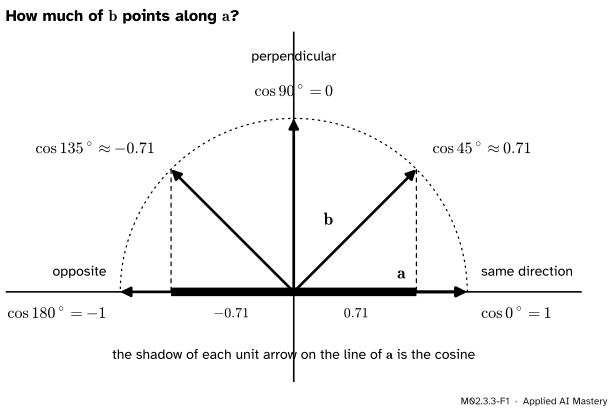
Take two arrows of length 1. The dot product is length times length times the cosine of the angle, and both lengths are 1. So for unit vectors the dot product is the cosine.
M02.3.3-F1
The cosine of the angle says how much of \(\vect{b}\) points along \(\vect{a}\). It is 1 when the two arrows agree, 0 when they are perpendicular and \(-1\) when they point in opposite directions.
For arrows of any length, divide the two lengths out of the dot product. What is left is the cosine of the angle. It runs from 1 (same direction) through 0 (perpendicular) to \(-1\) (opposite), and it does not change when either arrow is stretched. Used to compare data, this number is called the cosine similarity.
Build it up
Step 1. Solve for the cosine. The first lesson proved \(\vect{a} \cdot \vect{b} = \norm{\vect{a}}\,\norm{\vect{b}}\cos\theta\). For non-zero vectors, divide both sides by the two lengths:
Everything on the right comes from the coordinates. So an angle can be computed without a protractor: work out the fraction, then ask which angle has that cosine.
Step 2. Try it. For the module’s pair \(\vect{a} = (4, 2)\) and \(\vect{b} = (1, 3)\),
and the angle with that cosine is \(\theta = 45^\circ\).
Step 3. Normalise first, if you like. The same fraction is \(\frac{\vect{a}}{\norm{\vect{a}}} \cdot \frac{\vect{b}}{\norm{\vect{b}}}\), the dot product of the two unit vectors \(\hat{\vect{a}}\) and \(\hat{\vect{b}}\). Scale both arrows to length 1, then take a plain dot product.
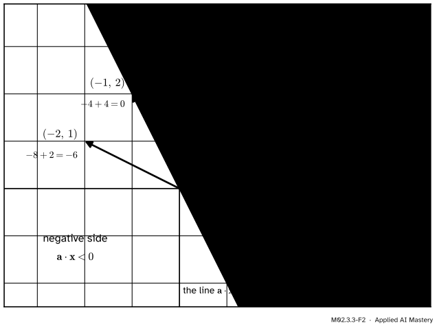
Step 4. Perpendicular means dot product zero. The cosine is 0 exactly at \(90^\circ\), and the fraction is 0 exactly when its top is 0. So two non-zero arrows are perpendicular exactly when \(\vect{a} \cdot \vect{b} = 0\). For example \((4, 2) \cdot (-1, 2) = -4 + 4 = 0\).
M02.3.3-F2
The vectors perpendicular to \(\vect{a}\) form a line through the origin. It splits the plane into a side where \(\vect{a} \cdot \vect{x}\) is positive and a side where it is negative.
The picture is also the simplest classifier in machine learning. A linear classifier keeps a weight vector \(\vect{w}\), computes \(\vect{w} \cdot \vect{x}\) for each input, adds a constant, and reads off the sign. In the plane its boundary is a line perpendicular to \(\vect{w}\).
Step 5. Is the fraction always a cosine? A cosine lies between \(-1\) and \(1\). In the plane we know the fraction is one, because we proved it. In 300 dimensions there is no protractor, and we would like to define the angle by this fraction. That is only safe if the top can never be bigger in size than the bottom. The guarantee is called the Cauchy-Schwarz inequality.
The formal statement
NoteResult: the Cauchy-Schwarz inequality
For all vectors \(\vect{a}\) and \(\vect{b}\) in \(\R^n\),
with equality exactly when one vector is a multiple of the other.
M02.3.3-F3
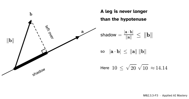
The picture behind the inequality. The shadow of \(\vect{b}\) on \(\vect{a}\) is one short side of a right triangle whose long side is \(\vect{b}\) itself, and a short side cannot be longer than the long side.
Proof. If \(\vect{a} = \vect{0}\), both sides are 0 and \(\vect{a} = 0\,\vect{b}\) is a multiple of \(\vect{b}\). So let \(\vect{a} \ne \vect{0}\). Pick any number \(t\) and look at the leftover \(\vect{b} - t\vect{a}\). A squared length is never negative, so
The last step multiplies out the brackets with the rules of the dot product. This holds for every \(t\). Now choose the \(t\) of the figure, the one that makes the leftover perpendicular to \(\vect{a}\):
Multiply by the positive number \(\vect{a} \cdot \vect{a}\) and move the last term across: \((\vect{a} \cdot \vect{b})^2 \le (\vect{a} \cdot \vect{a})(\vect{b} \cdot \vect{b}) = \norm{\vect{a}}^2\,\norm{\vect{b}}^2\). Take square roots, remembering that the square root of a square is an absolute value: \(\abs{\vect{a} \cdot \vect{b}} \le \norm{\vect{a}}\,\norm{\vect{b}}\).
Equality. With this \(t\) the calculation above is an exact identity: \(\norm{\vect{b} - t\vect{a}}^2 = \vect{b} \cdot \vect{b} - (\vect{a} \cdot \vect{b})^2 / (\vect{a} \cdot \vect{a})\). So the two sides of Cauchy-Schwarz are equal exactly when \(\norm{\vect{b} - t\vect{a}} = 0\), that is when \(\vect{b} = t\vect{a}\): nothing is left over, and \(\vect{b}\) lies along \(\vect{a}\).
For non-zero vectors \(\vect{a}\) and \(\vect{b}\) in \(\R^n\), the angle between them is the one number \(\theta\) from \(0^\circ\) to \(180^\circ\) with
That fraction is the cosine similarity of \(\vect{a}\) and \(\vect{b}\). Two vectors are orthogonal when \(\vect{a} \cdot \vect{b} = 0\).
Cauchy-Schwarz says the fraction lies between \(-1\) and \(1\), and every such number is the cosine of exactly one angle from \(0^\circ\) to \(180^\circ\). So the definition always makes sense. In the plane and in space it agrees with the protractor, by the first lesson. “Orthogonal” is the word for perpendicular that also works in 300 dimensions.
Three consequences, each used all the time.
Cosine similarity ignores length. Stretch the vectors by positive numbers \(k\) and \(m\). The top of the fraction becomes \(km\,(\vect{a} \cdot \vect{b})\) and the bottom becomes \(k\,\norm{\vect{a}} \cdot m\,\norm{\vect{b}}\). The factor \(km\) cancels, so the cosine is unchanged. A negative factor flips the arrow and with it the sign of the cosine.
Pythagoras, in any dimension. Multiply out \(\norm{\vect{a} + \vect{b}}^2 = (\vect{a} + \vect{b}) \cdot (\vect{a} + \vect{b}) = \norm{\vect{a}}^2 + 2\,\vect{a} \cdot \vect{b} + \norm{\vect{b}}^2\). So \(\norm{\vect{a} + \vect{b}}^2 = \norm{\vect{a}}^2 + \norm{\vect{b}}^2\) exactly when \(\vect{a} \cdot \vect{b} = 0\).
The triangle inequality, promised in the last lesson. Start from the same expansion:
The first \(\le\) holds because a number is at most its absolute value. The second is Cauchy-Schwarz. Both ends are squares of non-negative numbers, so taking square roots keeps the order: \(\norm{\vect{a} + \vect{b}} \le \norm{\vect{a}} + \norm{\vect{b}}\).
Frontier note: angles in high dimensions
In high dimensions almost every pair of directions is nearly perpendicular. Choose two directions in \(\R^n\) at random, every direction as likely as any other. By symmetry their cosine averages 0, and the average of its square is exactly \(1/n\). So its typical size is \(1/\sqrt{n}\): about 0.03 when \(n = 1000\) (Vershynin, High-Dimensional Probability, Section 3.3.3). A cosine of 0.3 between two embeddings with a thousand entries is about ten times that size, far more than two random directions would give.
Worked example
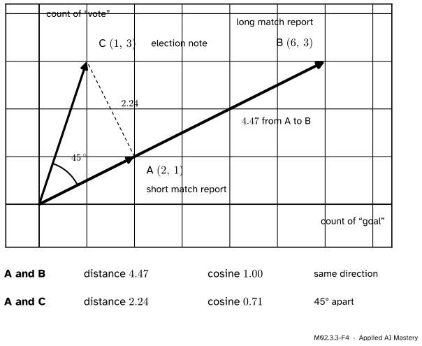
Three documents. Count two words in each: “goal” and “vote”. Document A, a short match report, has the count vector \(\vect{d}_A = (2, 1)\). Document B, a long match report, has \(\vect{d}_B = (6, 3)\). Document C, a note about an election, has \(\vect{d}_C = (1, 3)\). Which document is most like A?
M02.3.3-F4
Distance and cosine disagree. By distance the election note C is the nearer neighbour of A. By cosine the long match report B is a perfect match, because it points the same way.
By distance.\(\vect{d}_A - \vect{d}_B = (-4, -2)\), which has length \(\sqrt{16 + 4} = \sqrt{20} \approx 4.47\). And \(\vect{d}_A - \vect{d}_C = (1, -2)\), which has length \(\sqrt{1 + 4} = \sqrt{5} \approx 2.24\). Distance says C is closer.
By cosine. The lengths are \(\norm{\vect{d}_A} = \sqrt{5}\), \(\norm{\vect{d}_B} = \sqrt{45}\) and \(\norm{\vect{d}_C} = \sqrt{10}\). Write \(\cos(\vect{u}, \vect{v})\) for the cosine similarity of two vectors.
Cosine says B is a perfect match, at \(0^\circ\), and C is \(45^\circ\) away. That is the right answer for “same topic”: \(\vect{d}_B = 3\,\vect{d}_A\), the same mix of words, three times as long.
Orthogonal in space.\((1, 2, 2) \cdot (2, -2, 1) = 2 - 4 + 2 = 0\), so these two arrows are perpendicular. Pythagoras agrees: their sum \((3, 0, 3)\) has squared length 18, and \(\norm{(1, 2, 2)}^2 + \norm{(2, -2, 1)}^2 = 9 + 9 = 18\).
An obtuse angle. For \((4, 2)\) and \((-2, 1)\) the cosine is \(\frac{-6}{\sqrt{20}\,\sqrt{5}} = \frac{-6}{10} = -0.6\), which is an angle of about \(126.87^\circ\).
Code
From scratch. The angle function clips the cosine to the range \(-1\) to \(1\) first; the pitfalls explain why.
import mathdef dot(a, b):returnsum(x * y for x, y inzip(a, b))def norm(v):return math.sqrt(dot(v, v))def cosine(a, b):"""Cosine of the angle between two non-zero vectors."""if norm(a) ==0or norm(b) ==0:raiseValueError("the zero vector has no direction")return dot(a, b) / (norm(a) * norm(b))def angle_degrees(a, b): value =max(-1.0, min(1.0, cosine(a, b))) # clipped to the range -1 to 1return math.degrees(math.acos(value))print("a and b:", round(cosine((4, 2), (1, 3)), 4), round(angle_degrees((4, 2), (1, 3)), 2))A, B, C = (2, 1), (6, 3), (1, 3)print("A and B: distance", round(norm((A[0] - B[0], A[1] - B[1])), 2), " cosine", round(cosine(A, B), 4))print("A and C: distance", round(norm((A[0] - C[0], A[1] - C[1])), 2), " cosine", round(cosine(A, C), 4))print("in space:", cosine((1, 2, 2), (2, -2, 1)), angle_degrees((1, 2, 2), (2, -2, 1)))print("obtuse:", round(cosine((4, 2), (-2, 1)), 4), round(angle_degrees((4, 2), (-2, 1)), 2))
a and b: 0.7071 45.0
A and B: distance 4.47  cosine 1.0
A and C: distance 2.24  cosine 0.7071
in space: 0.0 90.0
obtuse: -0.6 126.87
The library version. scikit-learn compares every row of a table with every other row and returns a table of cosines.
import numpy as npfrom sklearn.metrics.pairwise import cosine_similaritydocs = np.array([[2.0, 1.0], # A: short match report [6.0, 3.0], # B: long match report [1.0, 3.0]]) # C: election notetable = cosine_similarity(docs)print(np.round(table, 4))unit = docs / np.linalg.norm(docs, axis=1, keepdims=True) # every row scaled to length 1print("same table from unit vectors:", np.allclose(unit @ unit.T, table))
[[1.     1.     0.7071]
 [1.     1.     0.7071]
 [0.7071 0.7071 1.    ]]
same table from unit vectors: True
A thousand random checks of the three results of this lesson, in seven dimensions.
rng = np.random.default_rng(0)for _ inrange(1000): a, b = rng.normal(size=(2, 7)) na, nb = np.linalg.norm(a), np.linalg.norm(b)assertabs(a @ b) <= na * nb +1e-12# Cauchy-Schwarzassert np.linalg.norm(a + b) <= na + nb +1e-12# triangle inequality k, m = rng.uniform(0.1, 10, size=2)assert np.isclose((k * a) @ (m * b) / (k * na * m * nb), a @ b / (na * nb)) # length is ignoredprint("Cauchy-Schwarz, the triangle inequality and scale-invariance hold on 1000 random pairs")
Cauchy-Schwarz, the triangle inequality and scale-invariance hold on 1000 random pairs
Two traps, shown once so that you recognise them.
from scipy.spatial.distance import cosine as cosine_distanceprint("SciPy's 'cosine' for A and C:", round(cosine_distance(docs[0], docs[2]), 4), " (1 minus the similarity)")ones = np.ones(3)raw = (ones @ ones) / (np.linalg.norm(ones) * np.linalg.norm(ones)) # the cosine of a vector with itselfprint("raw cosine:", repr(float(raw)), " (it should be 1; the last digit depends on the machine)")too_big =1.0000000000000002# the next number above 1with np.errstate(invalid="ignore"):print("arccos of", too_big, "is", np.arccos(too_big), " after clipping:", np.arccos(np.clip(too_big, -1, 1)))
SciPy's 'cosine' for A and C: 0.2929  (1 minus the similarity)
raw cosine: 1.0000000000000002  (it should be 1; the last digit depends on the machine)
arccos of 1.0000000000000002 is nan   after clipping: 0.0
Explore
This module’s interactive, the projection explorer, lives in the next lesson. Its read-out shows the angle and the cosine. Stretch either arrow and check that neither number moves. Then turn \(\vect{b}\) until the cosine is 0, and look at the dot product.
Pitfalls
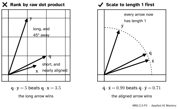
M02.3.3-F5
Wrong beside right. A raw dot product rewards length, so the long arrow \(\vect{y}\) outscores the well-aligned arrow \(\vect{x}\). Scale every arrow to length 1 first and the dot product becomes the cosine, which rewards direction only.
“The document with the largest dot product is the best match.”
A dot product grows with length. For the query \(\vect{q} = (2, 1)\), the long vector \(\vect{y} = (1, 3)\) scores \(2 + 3 = 5\) and the well-aligned \(\vect{x} = (1.5, 0.5)\) scores only \(3 + 0.5 = 3.5\). Their cosines tell the opposite story: \(0.71\) against \(0.99\). In text data, frequent words and long documents have long vectors, so a raw dot product favours them. If you want direction only, normalise first.
“A cosine similarity of 0 means the two vectors are opposites.”
Zero means perpendicular: the vectors have nothing in common. Opposite is \(-1\). With counts, which are never negative, a dot product cannot be negative either, so there the cosine runs only from 0 to 1 and 0 is the lowest score possible. Embeddings have negative entries and can use the whole range.
“Cosine similarity and cosine distance are the same thing.”
A similarity is large when two things are alike. A distance is small. scikit-learn’s cosine_similarity returns the cosine. SciPy’s distance.cosine returns 1 minus the cosine, so for documents A and C it prints \(0.2929\), not \(0.7071\). Sorting by the wrong one returns the worst matches first. And neither sees length: \((1, 1)\) and \((100, 100)\) have cosine 1.
“arccos returned nan, so the vectors must be broken.”
Rounding can push a computed cosine a hair outside the allowed range. For \((1, 1, 1)\) with itself the exact answer is 1, but the formula can return \(1.0000000000000002\). The last digit depends on the machine and the library, so never rely on it. arccos of any number above 1 is nan. Clip the cosine to the range \(-1\) to \(1\) before asking for the angle.
Check yourself
Recall
1. Write the formula for the cosine of the angle between two non-zero vectors.
2. How do you test whether two vectors are orthogonal?
Show answer
Compute their dot product. They are orthogonal exactly when it is zero.
3. State the Cauchy-Schwarz inequality.
Show answer
\(\abs{\vect{a} \cdot \vect{b}} \le \norm{\vect{a}}\,\norm{\vect{b}}\), with equality exactly when one vector is a multiple of the other.
4. What happens to the cosine similarity of \(\vect{a}\) and \(\vect{b}\) if you triple \(\vect{a}\)?
Show answer
Nothing. The factor 3 appears in the dot product and in the length of \(\vect{a}\), and cancels.
5. What cosine do two vectors have if they point the same way? If they are perpendicular? If they point in opposite directions?
Show answer
\(1\), \(0\) and \(-1\).
Exercises
1.★ Find the angle between (a) \((1, 0)\) and \((1, 1)\); (b) \((1, 2, 2)\) and \((2, 1, -2)\).
Show solution
(a) The dot product is 1 and the lengths are 1 and \(\sqrt{2}\), so \(\cos\theta = 1/\sqrt{2}\) and \(\theta = 45^\circ\).
(b) The dot product is \(2 + 2 - 4 = 0\). The vectors are orthogonal: \(\theta = 90^\circ\).
2.★★ A query has the word counts \(\vect{q} = (2, 2, 1)\). Two documents have \(\vect{d}_1 = (4, 4, 2)\) and \(\vect{d}_2 = (2, 1, 2)\). Rank the documents by distance from \(\vect{q}\), and then by cosine similarity with \(\vect{q}\). Which ranking would you trust for “same topic”, and why?
Show solution
Distance.\(\vect{q} - \vect{d}_1 = (-2, -2, -1)\) has length \(\sqrt{4 + 4 + 1} = 3\). \(\vect{q} - \vect{d}_2 = (0, 1, -1)\) has length \(\sqrt{2} \approx 1.41\). By distance, \(\vect{d}_2\) comes first.
Cosine.\(\norm{\vect{q}} = 3\), \(\norm{\vect{d}_1} = \sqrt{36} = 6\) and \(\norm{\vect{d}_2} = \sqrt{9} = 3\). Then \(\cos(\vect{q}, \vect{d}_1) = \frac{8 + 8 + 2}{3 \cdot 6} = \frac{18}{18} = 1\) and \(\cos(\vect{q}, \vect{d}_2) = \frac{4 + 2 + 2}{3 \cdot 3} = \frac{8}{9} \approx 0.89\). By cosine, \(\vect{d}_1\) comes first.
Trust the cosine. \(\vect{d}_1 = 2\vect{q}\) has exactly the same mix of words as the query and is simply twice as long. Distance punishes it for its length.
3.★★★ Let \(\hat{\vect{a}}\) and \(\hat{\vect{b}}\) be unit vectors with angle \(\theta\) between them. (a) Show that \(\norm{\hat{\vect{a}} - \hat{\vect{b}}}^2 = 2 - 2\cos\theta\). (b) Explain why, among unit vectors, the nearest neighbour by distance is also the best match by cosine.
The first and last terms are squared lengths of unit vectors, so each is 1. The middle term is \(-2\cos\theta\), because for unit vectors the dot product is the cosine. The total is \(2 - 2\cos\theta\).
(b) By (a), the squared distance is \(2 - 2\cos\theta\). As the cosine goes up, this goes down. So the unit vector with the largest cosine is the one with the smallest squared distance, and therefore the smallest distance. The two rankings are the same. So if every vector is normalised once, distance, dot product and cosine all give the same order.
Check with \(\hat{\vect{a}} = (1, 0)\) and \(\hat{\vect{b}} = (0, 1)\): the distance squared is \(1 + 1 = 2\), and \(2 - 2\cos 90^\circ = 2\).
Summary card
Divide the lengths out of a dot product and what is left is pure direction.
M02.3.3-F1
Cosine: from agree to oppose.
Angle.\(\cos\theta = \dfrac{\vect{a} \cdot \vect{b}}{\norm{\vect{a}}\,\norm{\vect{b}}}\), for non-zero vectors in any dimension.
Cosine similarity. The same fraction. It does not change when either vector is stretched.
Two consequences.\(\norm{\vect{a} + \vect{b}} \le \norm{\vect{a}} + \norm{\vect{b}}\), and \(\norm{\vect{a} + \vect{b}}^2 = \norm{\vect{a}}^2 + \norm{\vect{b}}^2\) exactly when \(\vect{a} \cdot \vect{b} = 0\).
Sources and next steps
Sources. Each was opened and checked against this lesson on 12 November 2026.
Sheldon Axler, Linear Algebra Done Right, 4th edition (open access). Section 6A: the definition of orthogonal (6.10), the Pythagorean theorem (6.12), the Cauchy-Schwarz inequality with its condition for equality (6.14) and the triangle inequality proved from it (6.17). Exercise 16 defines the angle in \(\R^n\) by the arccosine and asks why Cauchy-Schwarz is needed.
Marc Deisenroth, Aldo Faisal and Cheng Soon Ong, Mathematics for Machine Learning, Cambridge University Press, 2020 (free PDF). The Cauchy-Schwarz inequality (3.17), the angle defined through it (3.24 and 3.25) and orthogonality (Definition 3.7).
Daniel Jurafsky and James H. Martin, Speech and Language Processing, 3rd edition draft of 19 August 2026, chapter 5. Section 5.4, equations 5.7 to 5.10: the raw dot product favours long vectors, the normalised dot product is the cosine, for unit vectors the two coincide, and for non-negative counts the cosine runs from 0 to 1.
scikit-learn, cosine_similarity. The normalised dot product of the rows of two tables.
Roman Vershynin, High-Dimensional Probability, 2nd edition, Cambridge University Press, 2026 (free pre-publication PDF). Section 3.3.3, under “Isotropic random vectors are almost orthogonal”: for two independent random points \(X\) and \(Y\) of the unit sphere in \(\R^n\), the average of \((X \cdot Y)^2\) is \(1/n\), so the dot product is of size \(1/\sqrt{n}\) with high probability (equation 3.14). This is the frontier note.
Next.M02.3.4 Projection onto a line takes the shadow that appeared in the proof of Cauchy-Schwarz and makes it the main character.