Gram-Schmidt, written down as it runs, factors a matrix as A = QR: orthonormal columns times a triangle. Use the factorisation to project a vector onto a subspace and to fit the least-squares line through data, and check the answer against numpy.linalg.lstsq.
Record the Gram-Schmidt process as the factorisation A = QR, and explain why R is upper triangular.
Project a vector onto a subspace with an orthonormal basis, and prove that the projection is the closest point.
Fit a least-squares line by hand with QR and back substitution.
Compute the same fit with numpy.linalg.qr and numpy.linalg.lstsq, and reconcile a difference of signs.
In review. The maths and code on this page are checked by automated tests on every change, but an independent reader has not signed it off yet. Spot a mistake or a confusing step? Tell us.
The question
Four measurements, and a straight line with only two numbers to choose: no line passes through all four points. Which line is best? Every linear regression asks this question, and R’s lm function answers it with a factorisation called QR, which is the Gram-Schmidt process of the last lesson written as a product of two matrices. How does a recipe for perpendicular vectors fit a line to data?
From the last lesson
1. What are the two moves of the Gram-Schmidt process?
Show answer
Subtract from the new vector its shadows on all the directions already found, then scale what is left to length one.
2. What happens when one of the input vectors is a combination of the earlier ones?
Show answer
Nothing is left after the subtraction: \(\vect{e}_k = \vect{0}\), and it cannot be scaled to length one. The process has detected that the vectors are dependent.
Intuition
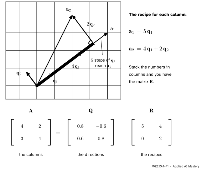
Gram-Schmidt computes more than the vectors \(\vect{q}_k\). Along the way it measures sizes: how long each shadow is, and how long each leftover is. Those numbers are worth keeping, because they say exactly how to rebuild every original vector from the \(\vect{q}\)’s.
For \(\vect{a}_1 = (4, 3)\) and \(\vect{a}_2 = (2, 4)\) the last lesson found a length of 5, a shadow of size 4 and a leftover of length 2. Read as recipes:
The factorisation \(\mat{A} = \mat{Q}\mat{R}\). The columns of \(\mat{Q}\) are the orthonormal directions, and each column of \(\mat{R}\) is the recipe for one column of \(\mat{A}\).
Put the \(\vect{q}\)’s in the columns of a matrix \(\mat{Q}\) and the recipes in the columns of a matrix \(\mat{R}\), and the two sentences above become one equation, \(\mat{A} = \mat{Q}\mat{R}\). This is the form in which orthonormal bases are used in practice, and its best-known job is fitting models to data.
Build it up
Step 1. Read Gram-Schmidt backwards. The process sets \(\vect{e}_k = \vect{a}_k - \sum_{j<k}{(\vect{q}_j \cdot \vect{a}_k)}\,\vect{q}_j\) and \(\vect{q}_k = \vect{e}_k / \norm{\vect{e}_k}\). Solve for \(\vect{a}_k\) and give the numbers names:
Step 2. Write it as a product. By the column rule of M02.5.2, column \(k\) of \(\mat{Q}\mat{R}\) is \(\mat{Q}\) times column \(k\) of \(\mat{R}\): a combination of the columns of \(\mat{Q}\) with those weights. Put \(r_{1k}, \dots, r_{kk}\) in column \(k\) of \(\mat{R}\), followed by zeros, and that combination is \(\vect{a}_k\). The zeros are there because \(\vect{a}_k\) needs only the first \(k\) directions. So \(\mat{R}\) has nothing below its diagonal: it is upper triangular.
Step 3. Mind the shapes. If \(\mat{A}\) has \(m\) rows and \(n\) columns, then \(\mat{Q}\) is also \(m \times n\), with \(\mat{Q}\T\mat{Q} = \mat{I}\), and \(\mat{R}\) is a small \(n \times n\) triangle. Multiplying \(\mat{A} = \mat{Q}\mat{R}\) on the left by \(\mat{Q}\T\) gives \(\mat{R} = \mat{Q}\T\mat{A}\): every entry of \(\mat{R}\) is one dot product, \(r_{jk} = {\vect{q}_j \cdot \vect{a}_k}\).
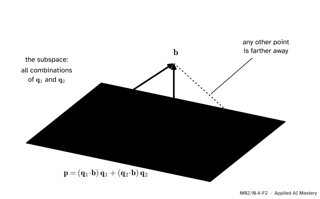
Step 4. The closest point of a subspace. Let \(\vect{q}_1, \dots, \vect{q}_n\) be orthonormal and let \(\vect{b}\) be a vector outside their span. Add up the shadows of \(\vect{b}\) on all of them:
The projection \(\vect{p}\) of \(\vect{b}\) onto a subspace is the sum of its shadows on an orthonormal basis. The error \(\vect{e} = \vect{b} - \vect{p}\) is perpendicular to the subspace, and that makes \(\vect{p}\) the closest point.
This \(\vect{p}\) is the projection of \(\vect{b}\) onto the subspace. It is what Gram-Schmidt subtracts at every step.
Step 5. Least squares. A system \(\mat{A}\vect{x} = \vect{b}\) with more equations than unknowns usually has no solution, because \(\vect{b}\) is not in the column space of \(\mat{A}\) (M02.7.2). The next best thing is the \(\hat{\vect{x}}\) for which \(\mat{A}\hat{\vect{x}}\) is the point of the column space closest to \(\vect{b}\). That point is \(\vect{p}\), and finding \(\hat{\vect{x}}\) takes one small triangular system.
The formal statement
Result 1: the QR factorisation. If the columns of an \(m \times n\) matrix \(\mat{A}\) are independent, then
\[
\mat{A} = \mat{Q}\mat{R},
\]
where \(\mat{Q}\) is \(m \times n\) with orthonormal columns and \(\mat{R}\) is \(n \times n\), upper triangular, with positive numbers on its diagonal.
Why. Steps 1 and 2 are the proof. The diagonal entries \(r_{kk} = \norm{\vect{e}_k}\) are positive by Claim 3 of the last lesson. Because they are not zero, any system \(\mat{R}\vect{x} = \vect{y}\) can be solved from the bottom row up by back substitution (M02.6.2), so \(\mat{R}\) is invertible.
Result 2: the projection is the closest point. Let \(S\) be the span of orthonormal vectors \(\vect{q}_1, \dots, \vect{q}_n\) in \(\R^m\), let \(\vect{b}\) be any vector of \(\R^m\), and put \(\vect{p} = \mat{Q}\mat{Q}\T\vect{b}\) and \(\vect{e} = \vect{b} - \vect{p}\).
(a) The error is perpendicular to \(S\). Dot \(\vect{e}\) with one basis vector:
In the sum, \({\vect{q}_j \cdot \vect{q}_i}\) is zero except for \(i = j\), when it is one. Every vector of \(S\) is a combination of the \(\vect{q}\)’s, so \(\vect{e}\) is perpendicular to all of \(S\).
(b) No point of \(S\) is closer. Take any \(\vect{w}\) in \(S\) and split the gap from \(\vect{w}\) to \(\vect{b}\) at \(\vect{p}\): \(\vect{b} - \vect{w} = \vect{e} + {(\vect{p} - \vect{w})}\). The second piece lies in \(S\), so it is perpendicular to \(\vect{e}\), and the cross term below is zero:
The last term is never negative, and it is zero only when \(\vect{w} = \vect{p}\). So the distance from \(\vect{b}\) to \(\vect{w}\) is smallest exactly at \(\vect{w} = \vect{p}\). \(\blacksquare\)
Result 3: least squares by QR. Let \(\mat{A} = \mat{Q}\mat{R}\) have independent columns. The \(\hat{\vect{x}}\) that makes \(\norm{\vect{b} - \mat{A}\vect{x}}\) as small as possible is the one solution of
Why. As \(\vect{x}\) varies, \(\mat{A}\vect{x}\) runs through the column space of \(\mat{A}\), which is the span of the \(\vect{q}\)’s (Claim 2 of the last lesson). By Result 2 the closest point to \(\vect{b}\) is \(\mat{Q}\mat{Q}\T\vect{b}\), so we need \(\mat{Q}\mat{R}\hat{\vect{x}} = \mat{Q}\mat{Q}\T\vect{b}\). Multiply on the left by \(\mat{Q}\T\) and use \(\mat{Q}\T\mat{Q} = \mat{I}\) on both sides: \(\mat{R}\hat{\vect{x}} = \mat{Q}\T\vect{b}\). In the other direction, multiplying that equation by \(\mat{Q}\) gives the first one back. Since \(\mat{R}\) is invertible there is exactly one \(\hat{\vect{x}}\).
The name least squares comes from what is minimised: \(\norm{\vect{b} - \mat{A}\vect{x}}^2\) is the sum of the squares of the gaps between the two sides of each equation.
Go deeper: the normal equations, and why QR is preferred
Result 2(a) says that the error is perpendicular to every column of \(\mat{A}\): \({\vect{a}_j \cdot {(\vect{b} - \mat{A}\hat{\vect{x}})}} = 0\) for each \(j\). Stacked up, those \(n\) equations read \(\mat{A}\T{(\vect{b} - \mat{A}\hat{\vect{x}})} = \vect{0}\), that is
These are the normal equations, and M03.7 studies them. They need no Gram-Schmidt, and on paper they give the same \(\hat{\vect{x}}\). On a computer they can fail. Forming \(\mat{A}\T\mat{A}\) multiplies the entries of \(\mat{A}\) by one another, so the small numbers that tell nearly parallel columns apart are squared and become far smaller still. Beside the large entries they are rounded away. The last code cell shows a matrix with independent columns whose computed \(\mat{A}\T\mat{A}\) is exactly singular. QR works on \(\mat{A}\) itself and does not have this problem.
Worked example
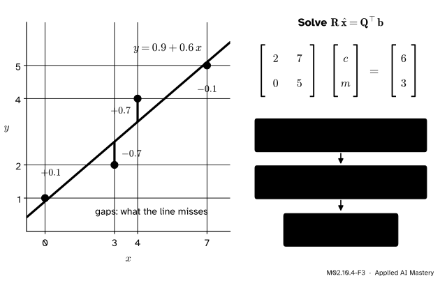
Fit the line \(y = c + m\,x\) to the points \((0, 1)\), \((3, 2)\), \((4, 4)\) and \((7, 5)\).
Asking the line to pass through all four points gives four equations in the unknowns \(c\) and \(m\):
There is no exact solution: the first two equations force \(c = 1\) and \(m = \tfrac13\), and then the third fails. So we look for the least-squares solution.
Gram-Schmidt on the two columns.\(\vect{a}_1 = (1, 1, 1, 1)\) has length \(\sqrt{4} = 2\), so \(r_{11} = 2\) and \(\vect{q}_1 = (0.5, 0.5, 0.5, 0.5)\). For \(\vect{a}_2 = (0, 3, 4, 7)\) the shadow has size \(r_{12} = {\vect{q}_1 \cdot \vect{a}_2} = {0.5 \cdot 14} = 7\), and
The bottom row says \(5m = 3\), so \(m = 0.6\). The top row says \(2c + {7 \cdot 0.6} = 6\), so \(2c = 1.8\) and \(c = 0.9\). The best line is \(y = 0.9 + 0.6\,x\).
Check. The line predicts \(\vect{p} = \mat{A}\hat{\vect{x}} = (0.9, 2.7, 3.3, 5.1)\), so the gaps are \(\vect{e} = \vect{b} - \vect{p} = (0.1, -0.7, 0.7, -0.1)\). They are perpendicular to both columns, as Result 2 demands:
The sum of squared gaps is \({0.01 + 0.49 + 0.49 + 0.01} = 1\), and no other line does better.
Code
From scratch: Gram-Schmidt that keeps its numbers, and back substitution.
import numpy as npdef qr_gram_schmidt(A):"""A = QR by Gram-Schmidt. Q has orthonormal columns; R is upper triangular.""" A = np.asarray(A, dtype=float) m, n = A.shape Q, R = np.zeros((m, n)), np.zeros((n, n))for k inrange(n): e = A[:, k].copy()for j inrange(k): R[j, k] = Q[:, j] @ A[:, k] # the size of the shadow on q_j e -= R[j, k] * Q[:, j] R[k, k] = np.linalg.norm(e) # the length of what is left Q[:, k] = e / R[k, k]return Q, Rdef back_substitute(R, y):"""Solve Rx = y for an upper-triangular R, from the bottom row up.""" n =len(y) x = np.zeros(n)for i inrange(n -1, -1, -1): x[i] = (y[i] - R[i, i +1:] @ x[i +1:]) / R[i, i]return xxs = np.array([0.0, 3.0, 4.0, 7.0])b = np.array([1.0, 2.0, 4.0, 5.0])A = np.column_stack([np.ones(4), xs])Q, R = qr_gram_schmidt(A)x_hat = back_substitute(R, Q.T @ b)print("R =\n", R)print("Q.T @ b =", Q.T @ b)print("intercept and slope:", x_hat)print("gaps:", np.round(b - A @ x_hat, 10), " sum of squares:", round(float(np.sum((b - A @ x_hat) **2)), 10))
R =
 [[2. 7.]
 [0. 5.]]
Q.T @ b = [6. 3.]
intercept and slope: [0.9 0.6]
gaps: [ 0.1 -0.7  0.7 -0.1]  sum of squares: 1.0
Now the library. numpy.linalg.qr returns the same factorisation up to signs, and numpy.linalg.lstsq solves the whole problem in one call.
Q_np, R_np = np.linalg.qr(A)print("NumPy's R =\n", np.round(R_np, 10))signs = np.sign(np.diag(R_np)) # flip so that the diagonal of R is positiveQ_fixed, R_fixed = Q_np * signs, signs[:, None] * R_npprint("same as ours after the flip:", np.allclose(Q_fixed, Q) and np.allclose(R_fixed, R))solution, squares, rank, _ = np.linalg.lstsq(A, b, rcond=None)print("lstsq:", solution, " sum of squared gaps:", squares)
NumPy's R =
 [[-2. -7.]
 [ 0. -5.]]
same as ours after the flip: True
lstsq: [0.9 0.6]  sum of squared gaps: [1.]
Here NumPy’s \(\mat{R}\) has a negative diagonal, the sign that LAPACK’s reflections usually give, although NumPy’s documentation promises no sign. It is still a correct factorisation: flip the sign of a column of \(\mat{Q}\) and of the matching row of \(\mat{R}\), and the product does not change.
Last, the warning of the “deeper” note: two columns that are independent but nearly parallel.
tiny =1e-8C = np.array([[1.0, 1.0], [tiny, 0.0], [0.0, tiny]])d = C @ np.array([1.0, 1.0]) # so the exact answer is (1, 1)print("rank of C:", np.linalg.matrix_rank(C), " rank of the computed C.T @ C:", np.linalg.matrix_rank(C.T @ C))Qc, Rc = np.linalg.qr(C)print("QR answer:", np.linalg.solve(Rc, Qc.T @ d))try: np.linalg.solve(C.T @ C, C.T @ d)except np.linalg.LinAlgError as error:print("normal equations:", error)
rank of C: 2   rank of the computed C.T @ C: 1
QR answer: [1. 1.]
normal equations: Singular matrix
In exact arithmetic \(\mat{C}\T\mat{C}\) has \(1 + 10^{-16}\) on its diagonal. A computer rounds that to 1, the matrix becomes singular, and the normal equations cannot be solved. QR returns \((1, 1)\).
Explore
The module’s interactive is the Gram-Schmidt stepper in lesson M02.10.3. Its read-out already speaks the language of this lesson: the size of each shadow and the length of each leftover are the entries of \(\mat{R}\). Step to the end with the starting vectors and read off \(5\), \(4\) and \(2\).
Pitfalls
M02.10.4-F4
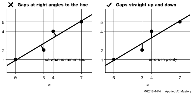
Wrong beside right. Least squares measures each gap vertically, as an error in \(y\) at a given \(x\). The right angle of this lesson is not in this picture at all: it sits in \(\R^4\), between the vector of gaps and the columns of \(\mat{A}\).
“The best line is the one closest to the points, measured at right angles.”
That is a different problem with a different answer. Least squares minimises the vertical gaps, because the equations compare \(y\)-values. For the four points above, the line that minimises the perpendicular distances has slope about \(0.618\), not \(0.6\). Minimising perpendicular distances is what principal component analysis does (M03.6).
“\(\mat{Q}\T\mat{Q} = \mat{I}\), so \(\mat{Q}\mat{Q}\T\vect{b}\) is just \(\vect{b}\).”
Only for a square \(\mat{Q}\). Here \(\mat{Q}\) is \(4 \times 2\), and \(\mat{Q}\mat{Q}\T\) is the \(4 \times 4\) matrix that projects onto the column space. It sends \(\vect{b} = (1, 2, 4, 5)\) to \((0.9, 2.7, 3.3, 5.1)\). If it returned \(\vect{b}\) unchanged, every data set would lie exactly on a line.
“NumPy’s Q and R have different signs from mine, so one of us is wrong.”
Both are right. A factorisation \(\mat{A} = \mat{Q}\mat{R}\) is unique only once the signs of the diagonal of \(\mat{R}\) are fixed. Gram-Schmidt makes them positive. NumPy’s routine does not promise a sign, and the second code cell shows how to flip one form into the other. The solution \(\hat{\vect{x}}\) is the same either way.
Check yourself
Recall
1. In \(\mat{A} = \mat{Q}\mat{R}\), what do the columns of \(\mat{Q}\) and of \(\mat{R}\) hold?
Show answer
The columns of \(\mat{Q}\) are the orthonormal vectors that Gram-Schmidt builds from the columns of \(\mat{A}\). Column \(k\) of \(\mat{R}\) holds the weights that rebuild \(\vect{a}_k\) from them: \(r_{jk} = {\vect{q}_j \cdot \vect{a}_k}\).
2. Why is \(\mat{R}\) upper triangular?
Show answer
Because \(\vect{a}_k\) is a combination of \(\vect{q}_1, \dots, \vect{q}_k\) only. The later \(\vect{q}\)’s are not needed, so the entries below the diagonal are zero.
3. What is the projection of \(\vect{b}\) onto the span of orthonormal vectors \(\vect{q}_1, \dots, \vect{q}_n\)?
Show answer
The sum of its shadows, \({(\vect{q}_1 \cdot \vect{b})}\vect{q}_1 + \cdots + {(\vect{q}_n \cdot \vect{b})}\vect{q}_n\), which is \(\mat{Q}\mat{Q}\T\vect{b}\). It is the point of the span closest to \(\vect{b}\).
4. Which small system gives the least-squares solution of \(\mat{A}\vect{x} = \vect{b}\)?
Show answer
\(\mat{R}\hat{\vect{x}} = \mat{Q}\T\vect{b}\), solved by back substitution.
5. When a line is fitted by least squares, which gaps are squared and added?
Show answer
The vertical gaps: the differences between each measured \(y\) and the line’s \(y\) at the same \(x\).
Exercises
1.★ Multiply \(\mat{Q} = \begin{bmatrix} 0.8 & -0.6 \\ 0.6 & 0.8 \end{bmatrix}\) by \(\mat{R} = \begin{bmatrix} 5 & 4 \\ 0 & 2 \end{bmatrix}\) and confirm that the product, call it \(\mat{A}\), has columns \((4, 3)\) and \((2, 4)\). Then compute \(\mat{Q}\T\mat{A}\).
Show solution
First column: \(5\,(0.8, 0.6) + 0\,(-0.6, 0.8) = (4, 3)\). Second column: \(4\,(0.8, 0.6) = (3.2, 2.4)\) plus \(2\,(-0.6, 0.8) = (-1.2, 1.6)\), which is \((2, 4)\). And
2.★★ Find the QR factorisation of the course’s running matrix \(\mat{A} = \begin{bmatrix} 1 & 1 \\ -1 & 2 \end{bmatrix}\). Multiply the diagonal entries of \(\mat{R}\), and explain why you get the area factor of \(\mat{A}\).
Show solution
\(\vect{a}_1 = (1, -1)\) has length \(\sqrt{2}\), so \(r_{11} = \sqrt{2}\) and \(\vect{q}_1 = \tfrac{1}{\sqrt{2}}(1, -1)\). For \(\vect{a}_2 = (1, 2)\), \(r_{12} = {\vect{q}_1 \cdot \vect{a}_2} = \tfrac{1}{\sqrt{2}}{(1 - 2)} = -\tfrac{1}{\sqrt{2}}\), and \(r_{12}\,\vect{q}_1 = -\tfrac12(1, -1)\). So \(\vect{e}_2 = (1, 2) + \tfrac12(1, -1) = (1.5, 1.5)\), of length \(r_{22} = 1.5\sqrt{2}\), and \(\vect{q}_2 = \tfrac{1}{\sqrt{2}}(1, 1)\):
The product of the diagonal is \({\sqrt{2} \cdot 1.5\sqrt{2}} = 3\), and \(\det\mat{A} = {1 \cdot 2} - {1 \cdot (-1)} = 3\). By the product rule, \(\det\mat{A} = \det\mat{Q}\,\det\mat{R}\). An orthogonal matrix has determinant \(\pm 1\) (here \(+1\): it is a rotation by \(-45°\)), and the determinant of a \(2 \times 2\) triangle is \(r_{11}r_{22} - 0\). In the picture, \(r_{11}\) is the base of the parallelogram spanned by the columns and \(r_{22}\) is its height.
3.★★★ Fit a line \(y = c + m\,x\) to the points \((0, 0)\), \((1, 1)\), \((2, 4)\) by QR. Then prove that the gaps of a least-squares line always add up to zero.
Show solution
Here \(\vect{a}_1 = (1, 1, 1)\), \(\vect{a}_2 = (0, 1, 2)\) and \(\vect{b} = (0, 1, 4)\). Gram-Schmidt gives \(r_{11} = \sqrt{3}\), \(\vect{q}_1 = \tfrac{1}{\sqrt{3}}(1, 1, 1)\), then \(r_{12} = \tfrac{3}{\sqrt{3}} = \sqrt{3}\), \(\vect{e}_2 = (0, 1, 2) - (1, 1, 1) = (-1, 0, 1)\), \(r_{22} = \sqrt{2}\) and \(\vect{q}_2 = \tfrac{1}{\sqrt{2}}(-1, 0, 1)\). The right-hand side is \({\vect{q}_1 \cdot \vect{b}} = \tfrac{5}{\sqrt{3}}\) and \({\vect{q}_2 \cdot \vect{b}} = \tfrac{4}{\sqrt{2}} = 2\sqrt{2}\).
Bottom row: \(\sqrt{2}\,m = 2\sqrt{2}\), so \(m = 2\). Top row: \(\sqrt{3}\,c + {\sqrt{3} \cdot 2} = \tfrac{5}{\sqrt{3}}\), so \(c + 2 = \tfrac53\) and \(c = -\tfrac13\). The line is \(y = -\tfrac13 + 2x\). It predicts \((-\tfrac13, \tfrac53, \tfrac{11}{3})\), so the gaps are \((\tfrac13, -\tfrac23, \tfrac13)\), which add up to zero.
Proof. By Result 2(a) the vector of gaps \(\vect{e}\) is perpendicular to every vector of the column space of \(\mat{A}\), and in particular to its first column \(\vect{a}_1 = (1, \dots, 1)\). But \({\vect{e} \cdot \vect{a}_1}\) is the sum of the entries of \(\vect{e}\). So the gaps add up to zero whenever the model has an intercept, because the intercept is what puts the column of ones into \(\mat{A}\).
Summary card
Gram-Schmidt, written down, is \(\mat{A} = \mat{Q}\mat{R}\).
M02.10.4-F1
Directions in Q, recipes in R.
Factorisation.\(\mat{A} = \mat{Q}\mat{R}\) with \(\mat{Q}\T\mat{Q} = \mat{I}\) and \(\mat{R} = \mat{Q}\T\mat{A}\) upper triangular.
Projection.\(\vect{p} = \mat{Q}\mat{Q}\T\vect{b}\) is the closest point of the column space to \(\vect{b}\).
Error.\(\vect{b} - \vect{p}\) is perpendicular to every column.
Least squares. Solve \(\mat{R}\hat{\vect{x}} = \mat{Q}\T\vect{b}\) by back substitution.
Sources and next steps
Sources. Each was opened and checked against this lesson on 12 November 2026.
David Austin, Understanding Linear Algebra, Section 6.4 and Section 6.5. Proposition 6.4.9 states the QR factorisation, Proposition 6.3.19 (in Section 6.3) the projection \(\mat{Q}\mat{Q}\T\vect{b}\), and Proposition 6.5.14 the least-squares solution \(\hat{\vect{x}} = \mat{R}^{-1}\mat{Q}\T\vect{b}\). Subsection 6.5.4 calls the QR route “numerically more reliable” than the normal equations.
Sheldon Axler, Linear Algebra Done Right, 4th edition (open access), Section 7D. Result 7.58 proves the QR factorisation of a square matrix from the Gram-Schmidt procedure, with positive numbers on the diagonal of \(\mat{R}\) and uniqueness.
Marc Deisenroth, Aldo Faisal and Cheng Soon Ong, Mathematics for Machine Learning, Section 3.8.2. Equation (3.56) is the normal equation, and equations (3.65) and (3.66) give the projection \(\mat{B}\mat{B}\T\vect{x}\) and its coordinates \(\mat{B}\T\vect{x}\) for an orthonormal basis.
Gilbert Strang, Projection matrices and least squares, MIT OpenCourseWare 18.06SC, lecture 16. Least squares “can be viewed as finding the projection of a vector”.
Dan Margalit and Joseph Rabinoff, Interactive Linear Algebra, Section 6.5. “The best-fit line minimizes the sum of the squares of these vertical distances.”
NumPy, numpy.linalg.qr and numpy.linalg.lstsq. The first returns “a matrix with orthonormal columns” and an upper-triangular matrix, and the page promises no sign. The second minimises the 2-norm of \(\vect{b} - \mat{A}\vect{x}\) and returns the sums of squared residuals.
The R Project, lm. The argument method: “for fitting, currently only method = "qr" is supported”.
Next. This lesson completes Linear Algebra I. Linear Algebra II starts with eigenvectors (M03.1) and returns to least squares, the normal equations and the pseudoinverse in M03.7.