Put an orthonormal basis in the columns of a matrix and you get a map that moves space rigidly. See why such a matrix satisfies Q-transpose times Q equals I, prove that it keeps every length and angle, and show that it is a rotation or a reflection whose inverse is its transpose.
Test whether a matrix is orthogonal by computing its transpose times itself, and explain each entry of that product as a dot product of two columns.
Prove that an orthogonal matrix keeps every dot product, every length and every angle.
Invert an orthogonal matrix by transposing it, and explain why that works.
Classify a 2 by 2 orthogonal matrix as a rotation or a reflection from its determinant.
In review. The maths and code on this page are checked by automated tests on every change, but an independent reader has not signed it off yet. Spot a mistake or a confusing step? Tell us.
The question
Turn a photograph and nothing in it is stretched: every length and every angle survives. Lesson M02.4.3 built the matrix of one rotation from its angle. But given only the numbers of a matrix, how can you tell that it moves space rigidly? And why do deep-learning libraries offer exactly these matrices as a way to set the starting weights of a network?
From the last lesson
1. In an orthonormal basis \(\vect{q}_1, \dots, \vect{q}_n\), what is the coordinate of \(\vect{v}\) along \(\vect{q}_i\)?
Show answer
The dot product \({\vect{v} \cdot \vect{q}_i}\). So \(\vect{v} = {(\vect{v} \cdot \vect{q}_1)}\vect{q}_1 + \cdots + {(\vect{v} \cdot \vect{q}_n)}\vect{q}_n\).
2. A vector has coordinates \((4, 2)\) in an orthonormal basis. What is its length?
Show answer
\(\sqrt{4^2 + 2^2} = \sqrt{20} \approx 4.47\). In an orthonormal basis the squared length is the sum of the squared coordinates.
Intuition
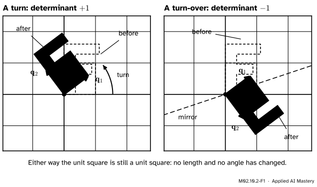
Take an orthonormal basis \(\vect{q}_1, \vect{q}_2\) and write the two vectors as the columns of a matrix \(\mat{Q}\). By M02.4.2, the columns of a matrix are where \(\ihat\) and \(\jhat\) land. So \(\mat{Q}\) sends the standard basis, two perpendicular arrows of length one, to \(\vect{q}_1\) and \(\vect{q}_2\), which are two perpendicular arrows of length one again. The unit square lands on a unit square. Nothing has been stretched, squashed or slanted. The plane has moved as one rigid sheet.
A rigid sheet pinned at the origin can move in only two ways. It can turn, or it can be turned over.
M02.10.2-F1
The two kinds of orthogonal matrix. Left: the columns \((0.8, 0.6)\) and \((-0.6, 0.8)\) turn the plane by about \(37°\). Right: the columns \((0.8, 0.6)\) and \((0.6, -0.8)\) reflect it in the dashed line, and the letter F comes out back to front.
A square matrix whose columns are orthonormal is called an orthogonal matrix. The name is a convention. “Orthonormal matrix” would describe it better, but nobody says that.
Build it up
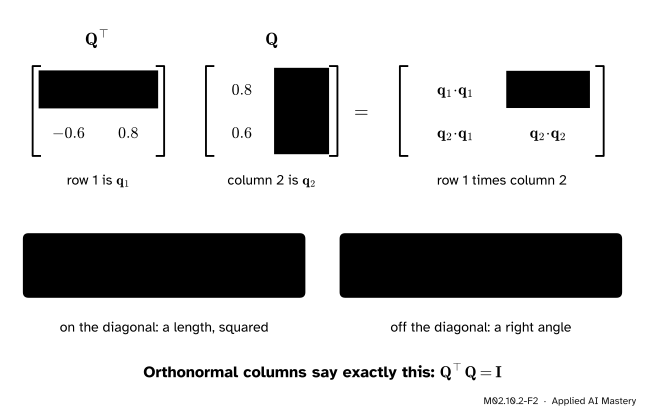
Step 1. The transpose. The transpose\(\mat{Q}\T\) of a matrix is the same numbers with rows and columns swapped: row \(i\) of \(\mat{Q}\T\) is column \(i\) of \(\mat{Q}\). If the columns of \(\mat{Q}\) are \(\vect{q}_1\) and \(\vect{q}_2\), then the rows of \(\mat{Q}\T\) are \(\vect{q}_1\) and \(\vect{q}_2\).
Step 2. Multiply \(\mat{Q}\T\) by \(\mat{Q}\). By the row-times-column rule of M02.5.2, the entry in row \(i\) and column \(j\) of a product is the dot product of row \(i\) of the first matrix with column \(j\) of the second. Here that is \({\vect{q}_i \cdot \vect{q}_j}\).
M02.10.2-F2
The product \(\mat{Q}\T\mat{Q}\) is a table of every dot product between the columns of \(\mat{Q}\). The diagonal holds the squared lengths, and everything off the diagonal tests a right angle.
So \(\mat{Q}\T\mat{Q}\) is the table of all dot products between the columns. “Orthonormal columns” says that this table has 1 down the diagonal and 0 everywhere else, which is the identity matrix \(\mat{I}\). One short equation, \(\mat{Q}\T\mat{Q} = \mat{I}\), carries every condition at once.
Step 3. Lengths survive. By the column view of M02.4.2, \(\mat{Q}\vect{x} = x_1\vect{q}_1 + x_2\vect{q}_2\). Read that sentence again: the entries of \(\vect{x}\) are the coordinates of \(\mat{Q}\vect{x}\) in the orthonormal basis \(\vect{q}_1, \vect{q}_2\). Result 4 of the last lesson reads a length off such coordinates: \(\norm{\mat{Q}\vect{x}}^2 = x_1^2 + x_2^2 = \norm{\vect{x}}^2\). The image has the length of the input.
Step 4. Transposing undoes it. Apply \(\mat{Q}\T\) to the image: \(\mat{Q}\T(\mat{Q}\vect{x}) = (\mat{Q}\T\mat{Q})\,\vect{x} = \mat{I}\vect{x} = \vect{x}\). We are back where we started. For this kind of matrix the inverse costs nothing to compute: swap rows and columns.
The formal statement
NoteDefinition: orthogonal matrix
A square matrix \(\mat{Q}\) is orthogonal if its columns are orthonormal. Equivalently,
\[
\mat{Q}\T\mat{Q} = \mat{I} .
\]
The two statements are the same because entry \((i, j)\) of \(\mat{Q}\T\mat{Q}\) is \({\vect{q}_i \cdot \vect{q}_j}\), as Step 2 showed. Four results follow. Let \(\mat{Q}\) be an \(n \times n\) orthogonal matrix with columns \(\vect{q}_1, \dots, \vect{q}_n\).
Result 1: dot products, lengths and angles are kept. For all vectors \(\vect{x}, \vect{y}\) in \(\R^n\),
Proof. Write both images by columns, \(\mat{Q}\vect{x} = \sum_i x_i\vect{q}_i\) and \(\mat{Q}\vect{y} = \sum_j y_j\vect{q}_j\), and expand the dot product into one term for each pair \((i, j)\):
The second line holds because \({\vect{q}_i \cdot \vect{q}_j}\) is 0 unless \(i = j\), when it is 1. \(\blacksquare\)
Two consequences. Put \(\vect{y} = \vect{x}\) to get \(\norm{\mat{Q}\vect{x}}^2 = \norm{\vect{x}}^2\): every length is kept. And the angle between two vectors is fixed by one dot product and two lengths, through \(\cos\theta = {\vect{x} \cdot \vect{y}} / (\norm{\vect{x}}\,\norm{\vect{y}})\) (M02.3.3). All three ingredients are unchanged, so every angle is kept too.
Result 2: the inverse is the transpose. The columns of \(\mat{Q}\) are orthonormal, so they are independent (Result 3 of the last lesson). Its null space is therefore only \(\vect{0}\) (M02.7.3), and a square matrix with that null space has an inverse (M02.7.4, proved there for every size). Multiply \(\mat{Q}\T\mat{Q} = \mat{I}\) on the right by that inverse, and use \(\mat{Q}\mat{Q}^{-1} = \mat{I}\):
It follows that \(\mat{Q}\mat{Q}\T = \mat{Q}\mat{Q}^{-1} = \mat{I}\) as well. Entry \((i, j)\) of \(\mat{Q}\mat{Q}\T\) is the dot product of rows \(i\) and \(j\) of \(\mat{Q}\), so the rows of an orthogonal matrix are orthonormal too. That is far from obvious from the definition.
Result 3: the determinant is \(+1\) or \(-1\). Take determinants of both sides of \(\mat{Q}\T\mat{Q} = \mat{I}\). By the product rule and \(\det(\mat{Q}\T) = \det(\mat{Q})\), both from M02.8.3,
so \(\det(\mat{Q}) = \pm 1\). Areas and volumes are kept, and the sign says whether space has been turned over.
Result 4: in the plane, a rotation or a reflection. Let \(\mat{Q}\) be \(2 \times 2\). Its first column is a unit vector, so it lies on the unit circle: \(\vect{q}_1 = (\cos\theta, \sin\theta)\) for some angle \(\theta\). Put \(\vect{n} = (-\sin\theta, \cos\theta)\). Then \({\vect{q}_1 \cdot \vect{n}} = -\cos\theta\sin\theta + \sin\theta\cos\theta = 0\) and \({\vect{n} \cdot \vect{n}} = \sin^2\theta + \cos^2\theta = 1\), so \(\vect{q}_1, \vect{n}\) is an orthonormal basis of the plane. Write the second column in that basis, using Result 1 of the last lesson:
where \(k = {\vect{q}_2 \cdot \vect{n}}\) and the first coordinate is zero because the columns are perpendicular. Since \(\vect{q}_2\) has length one, \(1 = \norm{k\,\vect{n}}^2 = k^2\), so \(k = 1\) or \(k = -1\). There are exactly two possibilities:
The first is the rotation matrix of M02.4.3, with determinant \(\cos^2\theta + \sin^2\theta = 1\). The second has determinant \(-\cos^2\theta - \sin^2\theta = -1\). It is a reflection in the line through the origin at angle \(\theta / 2\).
Go deeper: why the second matrix is a mirror
Call it \(\mat{F}\). Write \(\phi = \theta / 2\) for half the angle, so that \(\theta - \phi = \phi\), and let \(\vect{m} = (\cos\phi, \sin\phi)\) point along the claimed mirror line. Two formulas for the angle \(a - b\) are all we need:
\[
\begin{aligned}
\cos(a - b) &= \cos a\cos b \\
&\quad + \sin a\sin b, \\[0.3em]
\sin(a - b) &= \sin a\cos b \\
&\quad - \cos a\sin b .
\end{aligned}
\]
Multiply \(\mat{F}\) by \(\vect{m}\), row by row. The first entry of \(\mat{F}\vect{m}\), then the second, are
So \(\mat{F}\vect{m} = \vect{m}\): vectors along the line stay put. Now take \(\vect{p} = (-\sin\phi, \cos\phi)\), perpendicular to the line. The two entries of \(\mat{F}\vect{p}\) are
So \(\mat{F}\vect{p} = (\sin\phi, -\cos\phi) = -\vect{p}\). Every vector is a combination \(a\,\vect{m} + b\,\vect{p}\), and \(\mat{F}\) sends it to \(a\,\vect{m} - b\,\vect{p}\): the part along the line is kept and the part across it is reversed. That is a mirror. In more dimensions the split by determinant remains: orthogonal matrices with determinant \(+1\) are what “rotation” means in \(\R^n\), and those with determinant \(-1\) are a rotation combined with one reflection.
Frontier note: orthogonal weights keep signals alive in deep networks
A deep network multiplies its input by one weight matrix after another. If each matrix stretches vectors a little, the signal explodes with depth, and if each shrinks them a little, it dies away. The same happens to the gradients that flow backwards during training. An orthogonal matrix does neither, by Result 1. Saxe, McClelland and Ganguli (2013) studied deep linear networks and proposed random orthogonal matrices as starting weights, showing that they keep learning times independent of depth. Deep-learning libraries now ship this as a standard initialiser, for example torch.nn.init.orthogonal_ in PyTorch. The last code cell below shows the effect with fifty layers.
Worked example
Test \(\mat{Q} = \begin{bmatrix} 0.8 & -0.6 \\ 0.6 & 0.8 \end{bmatrix}\), then use it. Its columns are the basis \(\vect{q}_1 = (0.8, 0.6)\), \(\vect{q}_2 = (-0.6, 0.8)\) of the last lesson.
Is it orthogonal? The table \(\mat{Q}\T\mat{Q}\) needs three different dot products: \({\vect{q}_1 \cdot \vect{q}_1} = 0.64 + 0.36 = 1\), \({\vect{q}_2 \cdot \vect{q}_2} = 0.36 + 0.64 = 1\) and \({\vect{q}_1 \cdot \vect{q}_2} = -0.48 + 0.48 = 0\). So \(\mat{Q}\T\mat{Q} = \mat{I}\).
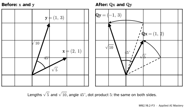
Apply it to two vectors. Take \(\vect{x} = (2, 1)\) and \(\vect{y} = (1, 3)\). By columns,
The matrix turns both vectors by the same angle. Each tip slides round a circle, so no length changes, and the two arrows keep the angle between them.
Compare before and after.
Quantity
Before
After
First squared length
\(2^2 + 1^2 = 5\)
\(1^2 + 2^2 = 5\)
Second squared length
\(1^2 + 3^2 = 10\)
\((-1)^2 + 3^2 = 10\)
Dot product
\({2 \cdot 1} + {1 \cdot 3} = 5\)
\({1 \cdot (-1)} + {2 \cdot 3} = 5\)
The cosine of the angle is \(5 / (\sqrt{5}\sqrt{10}) = 1/\sqrt{2}\) on both sides, an angle of \(45°\).
Undo it. The inverse is the transpose, so apply \(\mat{Q}\T\) to \((1, 2)\). The first entry is \({0.8 \cdot 1 + 0.6 \cdot 2} = 2\) and the second is \({-0.6 \cdot 1 + 0.8 \cdot 2} = 1\). That is \((2, 1)\), which is \(\vect{x}\) again.
Which kind is it?\(\det\mat{Q} = {0.8 \cdot 0.8} - (-0.6)(0.6) = 1\), so it is a rotation, by the angle with \(\cos\theta = 0.8\) and \(\sin\theta = 0.6\): about \(36.87°\).
Its mirror twin. Change the sign of the second column: \(\mat{F} = \begin{bmatrix} 0.8 & 0.6 \\ 0.6 & -0.8 \end{bmatrix}\) has determinant \({-0.64 - 0.36} = -1\). It keeps \((3, 1)\): the entries of \(\mat{F}(3, 1)\) are \({2.4 + 0.6} = 3\) and \({1.8 - 0.8} = 1\). It reverses \((-1, 3)\): the entries of \(\mat{F}(-1, 3)\) are \({-0.8 + 1.8} = 1\) and \({-0.6 - 2.4} = -3\). The mirror is the line through \((3, 1)\), at half the angle of the rotation.
Code
From scratch, with a matrix as a list of rows.
def transpose(M):return [list(column) for column inzip(*M)]def matmul(A, B):return [[sum(A[i][k] * B[k][j] for k inrange(len(B))) for j inrange(len(B[0]))]for i inrange(len(A))]def matvec(M, x):return [sum(m * xi for m, xi inzip(row, x)) for row in M]def dot(u, v):returnsum(a * b for a, b inzip(u, v))def is_orthogonal(M, tol=1e-12):"""Is M-transpose times M the identity?""" table = matmul(transpose(M), M)returnall(abs(table[i][j] - (1.0if i == j else0.0)) <= tolfor i inrange(len(M)) for j inrange(len(M)))Q = [[0.8, -0.6], [0.6, 0.8]]x, y = [2, 1], [1, 3]Qx, Qy = matvec(Q, x), matvec(Q, y)print("orthogonal:", is_orthogonal(Q))print("Qx, Qy:", [round(a, 10) for a in Qx], [round(a, 10) for a in Qy])print("dot products:", dot(x, y), round(dot(Qx, Qy), 10))print("undone:", [round(a, 10) for a in matvec(transpose(Q), Qx)])print("a shear is orthogonal:", is_orthogonal([[1, 1], [0, 1]]))
orthogonal: True
Qx, Qy: [1.0, 2.0] [-1.0, 3.0]
dot products: 5 5.0
undone: [2.0, 1.0]
a shear is orthogonal: False
The same checks with NumPy, and a function that names the kind of a 2 by 2 orthogonal matrix.
import numpy as npdef kind(M):"""Rotation or reflection, for a 2 by 2 orthogonal matrix."""assert np.allclose(M.T @ M, np.eye(2)), "not orthogonal"return"rotation"if np.linalg.det(M) >0else"reflection"Q = np.array([[0.8, -0.6], [0.6, 0.8]])F = np.array([[0.8, 0.6], [0.6, -0.8]])print("inverse equals transpose:", np.allclose(np.linalg.inv(Q), Q.T))print("rows orthonormal too: ", np.allclose(Q @ Q.T, np.eye(2)))turn = np.arctan2(Q[1, 0], Q[0, 0]) # the angle of the first column, in radiansprint("Q is a", kind(Q), "by", round(float(np.degrees(turn)), 2), "degrees")print("F is a", kind(F), "with determinant", round(float(np.linalg.det(F)), 10))
inverse equals transpose: True
rows orthonormal too:     True
Q is a rotation by 36.87 degrees
F is a reflection with determinant -1.0
Last, the claim of the frontier note. Send a vector of length one through fifty layers, three times: with random orthogonal matrices, and with random matrices whose entries are a little too large or a little too small.
from scipy.stats import ortho_grouprng = np.random.default_rng(0)n, depth =64, 50start = rng.normal(size=n)start /= np.linalg.norm(start) # a signal of length onedef length_after(make_layer): h = start.copy()for _ inrange(depth): h = make_layer() @ hreturnfloat(np.linalg.norm(h))orthogonal = length_after(lambda: ortho_group.rvs(n, random_state=rng))too_large = length_after(lambda: rng.normal(scale=1.2/ np.sqrt(n), size=(n, n)))too_small = length_after(lambda: rng.normal(scale=0.8/ np.sqrt(n), size=(n, n)))print(f"orthogonal layers: {orthogonal:.6f}")print(f"entries too large: {too_large:.0f}")print(f"entries too small: {too_small:.6f}")
orthogonal layers: 1.000000
entries too large: 3241
entries too small: 0.000007
After fifty orthogonal layers the length is still 1. The other two runs have grown into the thousands and shrunk to a few millionths.
Explore
This module’s interactive, the Gram-Schmidt stepper, lives in lesson M02.10.3. The two vectors it produces are the columns of an orthogonal matrix. While you are there, drag the second input across the first and watch that matrix switch between a rotation and a reflection.
Pitfalls
M02.10.2-F4
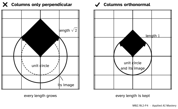
Wrong beside right. Perpendicular columns are not enough. On the left they have length \(\sqrt{2}\), and the map enlarges everything by that factor. Only on the right, where the columns also have length one, is every length kept.
“The columns are perpendicular, so the matrix is orthogonal.”
The name misleads. An orthogonal matrix needs orthonormal columns. The matrix with columns \((1, 1)\) and \((-1, 1)\) has perpendicular columns, but its table of dot products is \(2\,\mat{I}\), not \(\mat{I}\), and it stretches every vector by \(\sqrt{2}\). Divide it by \(\sqrt{2}\) and it becomes a rotation by \(45°\).
“Its determinant is 1, so it keeps lengths.”
Determinant \(\pm 1\) follows from being orthogonal, not the other way round. The shear \(\begin{bmatrix} 1 & 1 \\ 0 & 1 \end{bmatrix}\) has determinant 1 and keeps every area, yet it sends \((0, 1)\) to \((1, 1)\), of length \(\sqrt{2}\). Test \(\mat{Q}\T\mat{Q} = \mat{I}\), never the determinant alone.
“\(\mat{Q}\T\mat{Q} = \mat{I}\), so \(\mat{Q}\mat{Q}\T = \mat{I}\) as well.”
True for a square matrix, by Result 2. False for a tall one. The matrix with columns \((1, 0, 0)\) and \((0, 1, 0)\) has orthonormal columns, so \(\mat{Q}\T\mat{Q}\) is the \(2 \times 2\) identity. But \(\mat{Q}\mat{Q}\T\) is \(3 \times 3\) and sends \((x, y, z)\) to \((x, y, 0)\): it is a projection, not the identity. Lesson M02.10.4 puts that projection to work.
Check yourself
Recall
1. Which single equation says that a square matrix \(\mat{Q}\) is orthogonal?
Show answer
\(\mat{Q}\T\mat{Q} = \mat{I}\). It says that the columns of \(\mat{Q}\) are orthonormal.
2. What is the entry in row \(i\) and column \(j\) of \(\mat{Q}\T\mat{Q}\)?
Show answer
The dot product \({\vect{q}_i \cdot \vect{q}_j}\) of columns \(i\) and \(j\) of \(\mat{Q}\).
3. What is the inverse of an orthogonal matrix?
Show answer
Its transpose: \(\mat{Q}^{-1} = \mat{Q}\T\).
4. Name three things that an orthogonal matrix keeps unchanged.
Show answer
The dot product of any two vectors, the length of every vector, and the angle between any two vectors. Areas and volumes are kept as well, since the determinant is \(\pm 1\).
5. What can the determinant of an orthogonal matrix be, and what does each value mean in the plane?
Show answer
\(+1\) or \(-1\). In the plane, \(+1\) is a rotation and \(-1\) is a reflection.
Exercises
1.★ Show that \(\mat{M} = \dfrac{1}{13}\begin{bmatrix} 5 & -12 \\ 12 & 5 \end{bmatrix}\) is orthogonal. Write down its inverse, and say whether it is a rotation or a reflection.
Show solution
The columns are \(\tfrac{1}{13}(5, 12)\) and \(\tfrac{1}{13}(-12, 5)\). Each has squared length \({(25 + 144)}/169 = 1\), and their dot product is \({(-60 + 60)}/169 = 0\). So \(\mat{M}\T\mat{M} = \mat{I}\). The inverse is the transpose, \(\tfrac{1}{13}\begin{bmatrix} 5 & 12 \\ -12 & 5 \end{bmatrix}\). The determinant is \({(25 + 144)}/169 = 1\), so \(\mat{M}\) is a rotation, by the angle with \(\cos\theta = 5/13\) and \(\sin\theta = 12/13\), about \(67.4°\).
2.★★ The first column of a \(2 \times 2\) orthogonal matrix is \((0.6, 0.8)\). Find every possible second column, and describe the map each matrix performs.
Show solution
By Result 4 the second column is \(k\,(-0.8, 0.6)\) with \(k = \pm 1\).
With \(k = 1\) the matrix is \(\begin{bmatrix} 0.6 & -0.8 \\ 0.8 & 0.6 \end{bmatrix}\), with determinant \({0.36 + 0.64} = 1\): a rotation by the angle with \(\cos\theta = 0.6\), about \(53.13°\).
With \(k = -1\) it is \(\mat{F} = \begin{bmatrix} 0.6 & 0.8 \\ 0.8 & -0.6 \end{bmatrix}\), with determinant \(-1\): a reflection. Its mirror is at half that angle, along \((2, 1)\). Check: the entries of \(\mat{F}(2, 1)\) are \({1.2 + 0.8} = 2\) and \({1.6 - 0.6} = 1\), so \((2, 1)\) is kept. The entries of \(\mat{F}(-1, 2)\) are \({-0.6 + 1.6} = 1\) and \({-0.8 - 1.2} = -2\), so \((-1, 2)\) is reversed.
3.★★★ Suppose an \(n \times n\) matrix \(\mat{M}\) keeps every dot product: \({(\mat{M}\vect{x}) \cdot (\mat{M}\vect{y})} = {\vect{x} \cdot \vect{y}}\) for all \(\vect{x}, \vect{y}\). Show that \(\mat{M}\) is orthogonal. Deduce that the product of two orthogonal matrices is orthogonal.
Show solution
Choose \(\vect{x} = \vect{e}_i\) and \(\vect{y} = \vect{e}_j\), two standard basis vectors. Then \(\mat{M}\vect{e}_i\) is column \(i\) of \(\mat{M}\) (M02.4.2), call it \(\vect{m}_i\). The assumption gives \({\vect{m}_i \cdot \vect{m}_j} = {\vect{e}_i \cdot \vect{e}_j}\), which is 1 if \(i = j\) and 0 otherwise. So the columns of \(\mat{M}\) are orthonormal, and \(\mat{M}\) is orthogonal.
Now let \(\mat{Q}_1\) and \(\mat{Q}_2\) be orthogonal. Using Result 1 twice,
The first step applies Result 1 for \(\mat{Q}_1\) to the vectors \(\mat{Q}_2\vect{x}\) and \(\mat{Q}_2\vect{y}\), and the second applies it for \(\mat{Q}_2\). So \(\mat{Q}_1\mat{Q}_2\) keeps every dot product, and by the first part it is orthogonal. One rigid motion after another is a rigid motion.
Summary card
Orthonormal columns make a rigid motion: a turn or a turn-over.
M02.10.2-F1
Rotation or reflection, nothing stretched.
Test.\(\mat{Q}\T\mat{Q} = \mat{I}\): entry \((i, j)\) is \({\vect{q}_i \cdot \vect{q}_j}\).
Keeps.\({(\mat{Q}\vect{x}) \cdot (\mat{Q}\vect{y})} = {\vect{x} \cdot \vect{y}}\), so lengths and angles survive.
Inverse.\(\mat{Q}^{-1} = \mat{Q}\T\), and the rows are orthonormal too.
Determinant.\(\det\mat{Q} = \pm 1\): rotation for \(+1\), reflection for \(-1\) in the plane.
Sources and next steps
Sources. Each was opened and checked against this lesson on 12 November 2026.
Marc Deisenroth, Aldo Faisal and Cheng Soon Ong, Mathematics for Machine Learning, Section 3.4. Definition 3.8 defines an orthogonal matrix by equation (3.29), \(\mat{A}\mat{A}\T = \mat{I} = \mat{A}\T\mat{A}\), and (3.30) gives \(\mat{A}^{-1} = \mat{A}\T\). Equations (3.31) and (3.32) show that lengths and angles are kept. The margin note on the name “orthogonal” is on the same page.
Gilbert Strang, Orthogonal matrices and Gram-Schmidt, MIT OpenCourseWare 18.06SC, lecture 17. A full lecture on orthonormal vectors and orthogonal matrices, with a summary, problems and solutions.