Choose a penalty strength on validation data and report on a test set that is opened once. See by formula and by simulation how choosing on the test set makes the reported error too good, and treat the number of training steps as one more dial: early stopping.
Carry out the tuning routine: fit on training data, choose on validation data, report on test data once.
Explain why the best of several test scores is too good, and compute by how much in a simple case.
Measure by simulation how much choosing on the test set flatters the reported error.
Derive the shrinkage that early stopping applies to one weight and compare it with ridge.
Tune a penalty with scikit-learn’s GridSearchCV and stop gradient descent early from scratch.
In review. The maths and code on this page are checked by automated tests on every change, but an independent reader has not signed it off yet. Spot a mistake or a confusing step? Tell us.
The question
You try 45 settings of a model and report the lowest error any of them reached on the test set. Every step felt honest, yet the number is too good, and the more settings you try the more it flatters you. Where did the cheating happen? And what routine lets you tune as much as you like and still report an honest number?
From the last lesson
1. In k-fold cross-validation, how often is each example used to score a model?
Show answer
Exactly once, and always by a model that was fitted without it.
2. Why is the winner’s cross-validation error not an honest report of its quality?
Show answer
Because it was used to choose the winner. Part of its low value is luck, and the choosing kept the luck.
Intuition
Choosing is a kind of fitting. When you pick the price \(\lambda\) with the lowest validation error, you have fitted one number to the validation set. So the winner’s validation error flatters it a little, as a training error flatters a fitted model. That is harmless, provided one set of examples is left that never took part in any choice. That set is the test set, and it is opened once.
ML01.9.4-F1
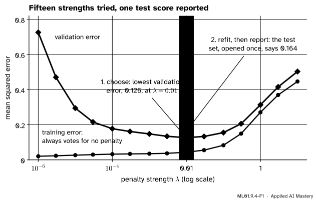
The routine on the dozen. Training error cannot choose the price. Validation error chooses \(\lambda = 0.01\). The test set is asked about that one model only.
At \(\lambda = 0.01\) the training error is \(0.043\) and the validation error \(0.126\). Refitted on all 24 examples, the model scores \(0.164\) on the test set, which took part in no decision.
Cross-validation, as in lesson 3, can do the choosing instead; the test set stays outside it.
Build it up
ML01.9.4-F2
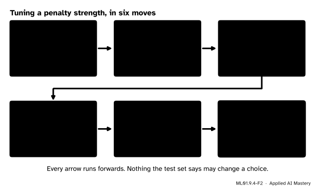
The test set appears in the last box only.
Step 1. Candidates. List the settings to try. For a price, use a grid that multiplies: here \(10^{-6}, 3 \times 10^{-6}, 10^{-5}, \dots, 3, 10\). A good price can lie anywhere over several powers of ten, and a grid that multiplies covers them with few candidates.
Step 2. Fit and score. Fit every candidate on the training set and score it on the validation set.
Step 3. Choose. Keep the candidate with the lowest score; if it sits at an end of the grid, extend the grid.
Step 4. Refit. Fit the winner again on training and validation examples together.
Step 5. Report. Compute the test error of that one model, and stop. Change anything because of it and test again, and the test set has become a validation set.
Step 6. Another dial. Gradient descent starts from small weights and grows them step by step, so stopping it early leaves them small, much as a penalty would. The number of updates is a setting like \(\lambda\) and is tuned the same way: watch the validation error while training and keep the weights from the step where it was lowest. This is early stopping.
The formal statement
NoteDefinition: the tuning routine
Split the examples into training, validation and test sets. For candidates \(1, \dots, M\):
fit each candidate on the training set;
choose \(\hat{\jmath}\), the candidate with the lowest validation error;
fit candidate \(\hat{\jmath}\) again, on the training and validation sets together;
report \(\closs{L_{\text{test}}}\) of that model, computed once.
Result 1: the best of several test scores is too good. Suppose step 2 chooses by test error instead, and that error is reported. Write \(T_j\) for the test error of candidate \(j\). It is a random number, because other test examples would have given another value, and its average \(\E[T_j] = e_j\) is the candidate’s true error. Let \(j^*\) be the truly best candidate. The reported number is the smallest score, and for every draw of the test set
Left: the reported error. Right: the true error of the chosen model. On average the report can only be too good: the argument of ML01.2.2 (Result 2), aimed at the test set. The honest routine escapes it because its model is fixed before the test set is opened, so that its test error is right on average.
Result 2: how much too good, in the simplest case. Let all \(M\) candidates be equally good, with true error \(e\). Let each test score be off by \(+s\) or \(-s\), as a fair coin decides, independently. The lowest score is \(e + s\) only if all \(M\) coins say \(+s\), which has probability \((\tfrac12)^M\). Otherwise it is \(e - s\). So
\[
\begin{aligned}
\E[\text{lowest}] &= \big(\tfrac12\big)^M (e + s) \\
&\quad + \Big(1 - \big(\tfrac12\big)^M\Big)(e - s) \\
&= e - s + 2s\,\big(\tfrac12\big)^M \\
&= e - s\,\big(1 - 2^{\,1 - M}\big) .
\end{aligned}
\]
With one candidate the report is right. With two it is too low by \(s/2\), with five by \(0.94\,s\), and soon by the full \(s\), though every candidate was the same.
Result 3: early stopping shrinks a weight. Take one centred feature and no penalty, and start gradient descent at \(w_0 = 0\). One update is
\[
\begin{aligned}
w &\leftarrow w - \eta\,(2w\,s_{xx} - 2s_{xy}) \\
&= m\,w + 2\eta\,s_{xy}, \\
m &= 1 - 2\eta\,s_{xx} .
\end{aligned}
\]
The update leaves the least-squares slope \(w_{\text{ls}} = s_{xy}/s_{xx}\) unchanged, because \(m\,w_{\text{ls}} = w_{\text{ls}} - 2\eta\,s_{xy}\). Subtract \(w_{\text{ls}}\) from both sides of the update: \(w - w_{\text{ls}} \leftarrow m\,(w - w_{\text{ls}})\), as in ML01.5.3. After \(t\) updates the starting distance \(0 - w_{\text{ls}}\) has been multiplied by \(m^t\):
Stopping after \(t\) updates multiplies the least-squares slope by \(1 - m^t\), where ridge multiplies it by \(s_{xx}/(s_{xx} + \lambda)\). Few updates act like a high price, many like a low one.
Go deeper: many weights: a rule of thumb linking steps and price
With several weights the same thing happens along each independent direction of the feature space, with its own variance in place of \(s_{xx}\). Directions in which the features vary a lot are learned in a few updates, those with little variance last, so stopping early leaves them out. Goodfellow, Bengio and Courville (Section 7.8) compare the two shrink factors direction by direction and find that they roughly agree when
\[
\lambda \approx \frac{1}{2\,\eta\,t} .
\]
It is a rough guide: on the four points below, \(t = 4\) and \(\eta = 0.1\) give \(1.25\) by the rule, while the exact match is \(\lambda = 0.58\).
Frontier note: tuning leaks at every scale
Cawley and Talbot (2010) showed that over-fitting the selection criterion can degrade a model surprisingly much, and that common ways of reporting results carry a selection bias. Their remedy is this lesson’s idea one level up, nested cross-validation: the whole tuning routine runs inside an outer loop of cross-validation.
Worked example
Part 1: tune the price on the dozen. Fifteen prices are fitted to the twelve training points; five of the rows:
\(\lambda\)
Training error
Validation error
\(10^{-6}\)
\(0.021\)
\(0.726\)
\(10^{-4}\)
\(0.033\)
\(0.177\)
\(0.01\)
\(0.043\)
\(0.126\)
\(1\)
\(0.271\)
\(0.313\)
\(10\)
\(0.446\)
\(0.503\)
Choose. The validation error is lowest at \(\lambda = 0.01\).
Refit. Fit that price again, to all 24 training and validation points.
Report. The test set, twelve further points from the same source (drawn with the validation points of lesson 1), gives that model \(0.164\): the number to report, not the validation error of \(0.126\), which was spent on the choice.
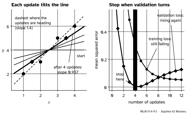
Part 2: early stopping on the four points. Start from the flat line at the mean, \(w = 0\) and \(b = 4\). With \(\eta = 0.1\), Result 3 gives \(m = 1 - 2 \times 0.1 \times 1.25 = 0.75\), so \(w_t = 1.4\,(1 - 0.75^t)\). Two more points, made up for this lesson, serve for validation: \((1.5, 3)\) and \((3.5, 5)\). The line \(\hat{y} = 4 + w\,(x - 2.5)\) predicts \(4 - w\) and \(4 + w\) for them, so their mean squared error is \((1 - w)^2\). The training loss is \(1.25w^2 - 3.5w + 2.5\) (lesson 1).
\(t\)
Slope \(w_t\)
Training loss
Validation loss
\(0\)
\(0\)
\(2.500\)
\(1.0000\)
\(1\)
\(0.3500\)
\(1.428\)
\(0.4225\)
\(2\)
\(0.6125\)
\(0.825\)
\(0.1502\)
\(3\)
\(0.8094\)
\(0.486\)
\(0.0363\)
\(4\)
\(0.9570\)
\(0.295\)
\(0.0018\)
\(5\)
\(1.0678\)
\(0.188\)
\(0.0046\)
\(6\)
\(1.1508\)
\(0.128\)
\(0.0227\)
The training loss falls at every update, towards \(0.05\) at \(w = 1.4\). The validation loss turns after update 4. Stop there, with \(w = 0.957\): the slope that ridge gives at \(\lambda = 0.58\), since \(1.75/0.957 - 1.25 = 0.58\).
ML01.9.4-F3
Left: every update tilts the line further towards the least-squares slope. Right: the training loss never stops falling; the validation loss is lowest after four updates.
Code
From scratch, with the refit and one look at the test set.
import numpy as npx_train = (np.arange(12) +0.5) /12y_train = np.array([0.18, 1.06, 0.84, 0.67, 0.33, -0.02, -0.40, -1.11, -0.66, -1.37, -0.38, -0.40])x_val = np.array([0.11, 0.34, 0.36, 0.37, 0.43, 0.58, 0.60, 0.75, 0.85, 0.87, 0.91, 0.98])y_val = np.array([0.93, 0.76, 0.45, 1.03, 0.11, -0.21, -0.23, -1.20, -0.88, -1.14, -0.89, -0.45])x_test = np.array([0.04, 0.15, 0.20, 0.23, 0.25, 0.42, 0.49, 0.61, 0.62, 0.80, 0.82, 0.97])y_test = np.array([0.55, 0.22, 1.42, 0.98, 0.61, 0.29, 0.05, -1.00, -0.13, -0.94, -0.46, 0.01])truth =lambda x: np.sin(2* np.pi * x) # the source of ML01.8; its noise has sd 0.3def powers(x, degree=9): u =2* x -1return np.column_stack([u ** k for k inrange(1, degree +1)])def fit_ridge(x, y, lam, degree=9): F = powers(x, degree) mu, sd = F.mean(axis=0), F.std(axis=0) Z, b, n = (F - mu) / sd, y.mean(), len(y) w = np.linalg.solve(Z.T @ Z / n + lam * np.eye(degree), Z.T @ (y - b) / n)returnlambda q: (powers(q, degree) - mu) / sd @ w + bmse =lambda predict, x, y: float(np.mean((predict(x) - y) **2))true_error =lambda predict: mse(predict, x_test, truth(x_test)) +0.3**2# averaged over endless fresh targetsgrid = np.array([m *10.0** e for e inrange(-6, 1) for m in (1, 3)] + [10.0])models = [fit_ridge(x_train, y_train, lam) for lam in grid] # 1. fit each candidateval = np.array([mse(p, x_val, y_val) for p in models])chosen =int(val.argmin()) # 2. choose on validationprint(f"chosen price {grid[chosen]:g}: training {mse(models[chosen], x_train, y_train):.3f}, "f"validation {val[chosen]:.3f}")x_pool, y_pool = np.concatenate([x_train, x_val]), np.concatenate([y_train, y_val])final = fit_ridge(x_pool, y_pool, grid[chosen]) # 3. refit on all 24print(f"test error of the refitted model: {mse(final, x_test, y_test):.3f}") # 4. report, onceprint(f"true error: {true_error(models[chosen]):.3f} before the refit, {true_error(final):.3f} after")
chosen price 0.01: training 0.043, validation 0.126
test error of the refitted model: 0.164
true error: 0.127 before the refit, 0.110 after
The last line is a luxury of a made-up source: over endless fresh targets at the test inputs, the refit cut the error from \(0.127\) to \(0.110\). Yet on these twelve test points the two models score within \(0.001\) of each other: a test score is itself a noisy measurement (ML01.2.3).
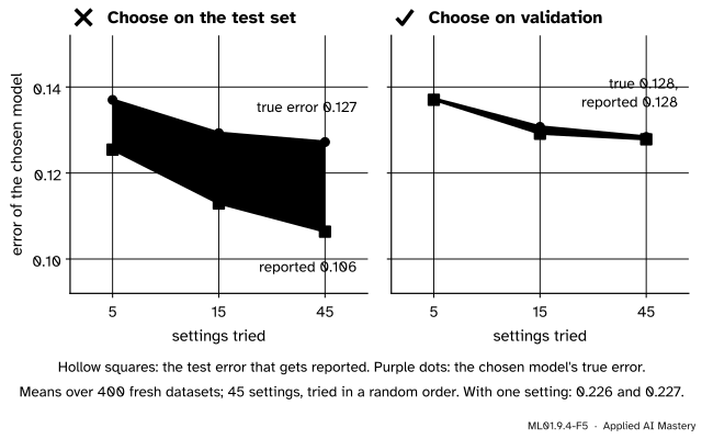
Now cheat on purpose. Each round draws fresh targets for all three sets and fits 45 settings, nine degrees times five prices. A peeker tries the first \(M\) settings of a random order and reports the lowest test error. An honest tuner tries the same \(M\), chooses on validation, and reports that one model’s test error.
settings = [(degree, lam) for degree inrange(1, 10) for lam in (1e-4, 1e-3, 1e-2, 1e-1, 1.0)]counts = [1, 5, 15, 45]rng = np.random.default_rng(0)log = {M: [] for M in counts}for _ inrange(400): y_tr, y_va, y_te = (truth(x) +0.3* rng.normal(size=12) for x in (x_train, x_val, x_test)) fits = [fit_ridge(x_train, y_tr, lam, degree) for degree, lam in settings] val_err = np.array([mse(p, x_val, y_va) for p in fits]) test_err = np.array([mse(p, x_test, y_te) for p in fits]) true_err = np.array([true_error(p) for p in fits]) order = rng.permutation(len(settings))for M in counts: tried = order[:M] peek, fair = tried[test_err[tried].argmin()], tried[val_err[tried].argmin()] log[M].append((test_err[peek], true_err[peek], test_err[fair], true_err[fair]))for M in counts: a = np.mean(log[M], axis=0)print(f"{M:2d} settings: peeker reports {a[0]:.3f}, truth {a[1]:.3f} | honest reports {a[2]:.3f}, truth {a[3]:.3f}")
 1 settings: peeker reports 0.226, truth 0.227   |   honest reports 0.226, truth 0.227
 5 settings: peeker reports 0.125, truth 0.137   |   honest reports 0.137, truth 0.137
15 settings: peeker reports 0.113, truth 0.129   |   honest reports 0.129, truth 0.131
45 settings: peeker reports 0.106, truth 0.127   |   honest reports 0.128, truth 0.128
With one setting both reports are right. With 45, the peeker reports \(0.106\) for a model whose true error is \(0.127\): a sixth too good. The honest tuner reports \(0.128\) for a model worth \(0.128\). Their models are equally good, but only one of them knows it.
Early stopping on the dozen, with the validation error checked at every update.
F = powers(x_train)mu, sd = F.mean(axis=0), F.std(axis=0)Z, Z_val, b = (F - mu) / sd, (powers(x_val) - mu) / sd, y_train.mean()w, history = np.zeros(9), []for step inrange(100_000): w = w -0.1*2* Z.T @ (Z @ w + b - y_train) /12# one plain update, learning rate 0.1 history.append(np.mean((Z_val @ w + b - y_val) **2))history = np.array(history)best_step =int(history.argmin()) +1print(f"lowest validation error {history.min():.3f}, after {best_step} updates")for steps in [10, 100, 1000, 10_000, 100_000]:print(f"after {steps:>7,} updates: validation error {history[steps -1]:.3f}")w4 = [1.4* (1-0.75** t) for t inrange(7)] # the four points, by Result 3print("four points:", np.round(w4, 4), " validation loss:", np.round([(1- s) **2for s in w4], 4))
lowest validation error 0.126, after 316 updates
after      10 updates: validation error 0.205
after     100 updates: validation error 0.135
after   1,000 updates: validation error 0.138
after  10,000 updates: validation error 0.165
after 100,000 updates: validation error 0.203
four points: [0.     0.35   0.6125 0.8094 0.957  1.0678 1.1508]  validation loss: [1.     0.4225 0.1502 0.0363 0.0018 0.0046 0.0227]
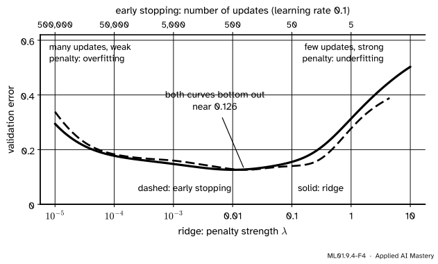
The validation error falls to \(0.126\) after 316 updates, the value the best ridge price reached, and then climbs slowly towards the \(1.18\) of the unpenalised fit.
ML01.9.4-F4
Two dials, one effect: the validation error of ridge against its price and of early stopping against its number of updates, the axes lined up by \(\lambda \approx 1/(2\eta t)\).
The library’s GridSearchCV cross-validates every candidate, keeps the best, and refits it on all the data it was given. The test set is not given to it.
chosen price: 0.01  cross-validation error: 0.149
test error, opened once: 0.165
KFold’s own folds choose \(\lambda = 0.01\) again, with a cross-validation error of \(0.149\) where lesson 3’s folds gave \(0.108\). One detail: alpha is \(n\lambda\), and the refit keeps alpha\(= 0.18\) for all 24 examples, which is our \(\lambda = 0.0075\). Hence a test error of \(0.165\) where ours was \(0.164\).
Explore
The penalty explorer of lesson 2 shows steps 1 to 3 of the routine live: slide the price, read the validation error, press Lowest validation error. It shows no test set, on purpose: you would tune by it.
Pitfalls
ML01.9.4-F5
Wrong beside right. Left: choosing by test error: the more settings are tried, the further the report sinks below the truth. Right: choosing by validation error and testing once: the report is right on average, however many settings are tried.
“I never trained on the test set. I only used it to pick the best setting.”
Picking is fitting. The peeker never trained on a test example, and still reported \(0.106\) for a model worth \(0.127\). By Result 2 the gap would exist even if every setting were equally good.
“The test score was disappointing, so I adjusted the model and tested again.”
Now two models have been compared on the test set and the better kept: choosing by test error with \(M = 2\). To keep improving, return to the validation data, and find fresh test examples for the final report.
“Train until the training loss stops falling.”
On the dozen the validation error had been rising since update 316 while the training loss was still creeping down after 100,000. The training loss cannot say when to stop, for the same reason that it cannot choose \(\lambda\).
Check yourself
Recall
1. Which set does each job in the tuning routine: fitting, choosing, reporting?
Show answer
The training set fits, the validation set (or cross-validation) chooses, and the test set reports on the chosen model, once.
2. Why is the lowest of several test errors too good on average?
Show answer
Each test error is a true error plus luck. Taking the lowest favours good luck, so the minimum averages below the true error of even the best candidate.
3. In the coin model with \(M\) equally good candidates, what is the expected lowest score?
Show answer
\(e - s\,(1 - 2^{1-M})\): right for \(M = 1\), too low by \(s/2\) for \(M = 2\), and close to \(e - s\) for large \(M\).
4. What is early stopping, and which set decides when to stop?
Show answer
Stopping gradient descent at the update where the validation error is lowest, long before the training loss is. The validation set decides.
5. After \(t\) updates from \(w = 0\), by what factor has early stopping shrunk a single least-squares weight?
Show answer
By \(1 - m^t\) with \(m = 1 - 2\eta\,s_{xx}\): near 0 after few updates, near 1 after many.
Exercises
1.★ A colleague shows you this table and reports “error 0.21”. What should have been reported, and what else would you ask?
Setting
Validation error
Test error
A
\(0.30\)
\(0.33\)
B
\(0.24\)
\(0.29\)
C
\(0.26\)
\(0.21\)
Show solution
The validation error chooses B, so the report should be B’s test error, \(0.29\). The reported \(0.21\) is the lowest test error, that of C: the setting was chosen by peeking. And ask why A and C were tested at all.
2.★★ Run early stopping on the four points with \(\eta = 0.2\). Find \(w_3\), the shrinkage it has applied, and the ridge price that gives the same slope.
Show solution
\(m = 1 - 2 \times 0.2 \times 1.25 = 0.5\), so \(w_t = 1.4\,(1 - 0.5^t)\) and \(w_3 = 1.4 \times 0.875 = 1.225\). The shrink factor is \(1 - 0.5^3 = 0.875\). Ridge gives the same slope when \(1.75/(1.25 + \lambda) = 1.225\), so \(1.25 + \lambda = 1.4286\) and \(\lambda = 0.179\).
3.★★★ Ten settings are equally good, with true error \(0.30\). On your test set each one’s score is \(0.30 \pm 0.04\), by a fair coin, independently. What is the expected value of the best score? How many settings would it take for the best score to average below \(0.265\)?
Show solution
By Result 2 with \(e = 0.30\), \(s = 0.04\) and \(M = 10\): \(0.30 - 0.04\,(1 - 2^{-9}) = 0.30 - 0.04 \times 0.998 = 0.2601\). For the average to be below \(0.265\) we need \(0.04\,(1 - 2^{1-M}) > 0.035\), so \(1 - 2^{1-M} > 0.875\), so \(2^{1-M} < 0.125 = 2^{-3}\), so \(M > 4\). Five settings are enough: \(0.30 - 0.04 \times 0.9375 = 0.2625\).
Summary card
Fit on training data, choose on validation data, and open the test set once.
Why.\(\E[\min_j T_j] \le e_{j^*} \le \E[e_{\hat{\jmath}}]\): the best of several test scores is too good.
Coin model. With \(M\) equal candidates the best score averages \(e - s\,(1 - 2^{1-M})\).
Measured. 45 settings: a peeker reports \(0.106\) for a true \(0.127\), an honest tuner \(0.128\) for \(0.128\).
Early stopping.\(w_t = {(1 - m^t)}\,w_{\text{ls}}\) with \(m = 1 - 2\eta\,s_{xx}\): few updates act like a high price.
The dozen.\(\lambda = 0.01\): validation \(0.126\), test \(0.164\). Early stopping: \(0.126\) after 316 updates.
Sources and next steps
Sources. Each was opened and checked against this lesson on 12 November 2026.
Trevor Hastie, Robert Tibshirani and Jerome Friedman, The Elements of Statistical Learning, 2nd edition (free PDF from the authors). Section 7.2 assigns model selection to the validation set and model assessment to the test set, which should be kept in a “vault”: used repeatedly to choose the model with the smallest test error, that error “will underestimate the true test error, sometimes substantially”. Section 11.5.2 describes early stopping, with a validation set to decide when to stop.
Ian Goodfellow, Yoshua Bengio and Aaron Courville, Deep Learning, MIT Press, 2016, Section 7.8. Treats the number of training steps as “just another hyperparameter” with a U-shaped validation curve, and shows that under a quadratic approximation early stopping is equivalent to L2 regularisation, with about \(1/(\epsilon\alpha)\) steps (equation 7.44) for learning rate \(\epsilon\) and penalty \(\frac{\alpha}{2}w^2\). Their \(\alpha\) is our \(2\lambda\).
scikit-learn 1.9 API reference, GridSearchCV. An exhaustive search over given parameter values, by 5-fold cross-validation by default; with refit=True, the default, it refits the best setting on the whole dataset.
Gavin Cawley and Nicola Talbot, On Over-fitting in Model Selection and Subsequent Selection Bias in Performance Evaluation, Journal of Machine Learning Research 11 (2010), pages 2079 to 2107. The abstract states that over-fitting the model selection criterion can degrade performance surprisingly much and that common evaluation practices are susceptible to selection bias; the introduction recommends nested cross-validation.
Next. Module ML01.10, A full project from raw data to report, uses everything in this module on a real dataset: a pipeline, a tuned penalty, cross-validation, and one look at the test set at the very end.