One validation set is a small jury, and the examples in it never help to fit. k-fold cross-validation lets every example do both jobs in turn. Work it fold by fold by hand, build it from scratch in NumPy, match scikit-learn, and count what it costs.
Carry out k-fold cross-validation by hand on a small dataset, fold by fold.
Show that with equal folds the cross-validation error scores every example exactly once.
Explain why cross-validation uses the data better than a single split, and count the fits it costs.
Choose a penalty strength by cross-validation from scratch in NumPy and with scikit-learn.
Keep every step that learns from the data inside the folds.
In review. The maths and code on this page are checked by automated tests on every change, but an independent reader has not signed it off yet. Spot a mistake or a confusing step? Tell us.
The question
Of the three prices lesson 1 tried, \(\lambda = 0.01\) scored best on twelve validation points. Twelve is a small jury: a different twelve might have voted another way. And those twelve never helped to fit anything, which is a waste when there are only twenty-four examples in all. Can every example sit on the jury and help to fit, without ever judging a model it helped to build?
From the last lesson
1. What does soft thresholding do to a least-squares weight?
Show answer
It moves the weight towards zero by a fixed amount and stops at zero, so a small enough weight becomes exactly zero.
2. Why does the lasso produce exact zeros and ridge does not?
Show answer
The lasso’s price \(\abs{w}\) is as steep at zero as anywhere, so a weak feature is not worth its first crumb of weight. The ridge price \(w^2\) is flat at zero, so some weight always pays.
Intuition
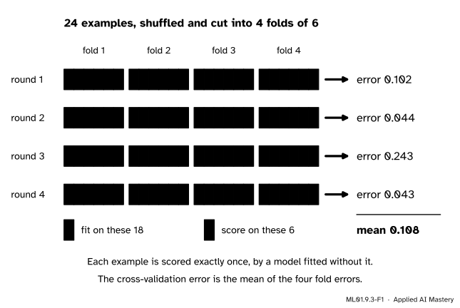
Take turns. Shuffle the examples and cut them into a few equal groups, called folds. Hold the first fold out, fit on the others, and score the model on the fold it never saw. Put that fold back, hold out the second, and repeat. When every fold has had its turn, average the scores. This is k-fold cross-validation, with \(k\) the number of folds.
ML01.9.3-F1
Four-fold cross-validation of ridge with \(\lambda = 0.01\) on 24 examples. Each round fits on 18 examples and scores on the 6 held out. No example is ever scored by a model that saw it.
Three things have improved on the single split of lesson 1. Each model is fitted to 18 examples instead of 12. All 24 examples judge instead of 12. And the verdict no longer hangs on one draw of the jury: the four rounds disagree, from \(0.043\) to \(0.243\), and any one of them alone would have been the “validation error” of some single split.
Build it up
Step 1. Shuffle, then cut. Shuffle the example numbers with a seed, as in ML01.2.2, and cut the shuffled row into \(k\) folds of equal size.
Step 2. One round per fold. In round \(j\), fold \(j\) is the validation set and the other \(k - 1\) folds together are the training set. Fit, then compute the error on fold \(j\).
Step 3. Average. The cross-validation error is the mean of the \(k\) fold errors.
Step 4. Choose. Do all of that for each candidate, here each price \(\lambda\), using the same folds every time. Keep the candidate with the lowest cross-validation error.
Step 5. Refit. The \(k\) models of each candidate were each fitted to part of the data. Throw them away, and fit the winning candidate once more, on everything.
Step 6. Pay. Each candidate costs \(k\) fits instead of one.
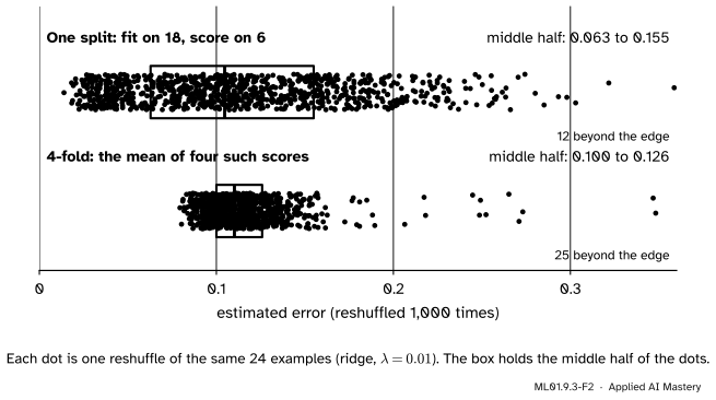
How much steadier is the verdict? Reshuffle the same 24 examples a thousand times.
ML01.9.3-F2
A thousand reshuffles. The middle half of the single-split estimates spans \(0.063\) to \(0.155\). The middle half of the four-fold estimates spans \(0.100\) to \(0.126\), less than a third as wide.
Both rows have strays far to the right: shuffles in which an end point of the input range was held out, so that the polynomial had to guess beyond its data.
The formal statement
NoteDefinition: k-fold cross-validation
Sort the example numbers \(1, \dots, n\) into \(k\) folds \(F_1, \dots, F_k\), so that each number is in exactly one fold. Write \(\cmodel{f^{(-j)}}\) for the model fitted to every example except those in \(F_j\). The error of fold \(j\) and the cross-validation error are
The first line puts \(n/k\) for \(\abs{F_j}\), and the second cancels \(k\). Every example lies in exactly one fold, so the double sum visits each example once: a mean squared error over all\(n\) examples, each predicted by a model that never saw it.
Result 2: the count. Each round fits on the other \(k - 1\) folds, that is on \(n\,(k - 1)/k\) examples. Over the \(k\) rounds each example is in the training set \(k - 1\) times and in the validation set once. With \(M\) candidates the bill is \(kM\) fits, plus one final refit.
Choosing \(k\). Common choices are \(k = 5\) and \(k = 10\). A larger \(k\) gives each model more examples and costs more fits. The largest, \(k = n\), holds out one example at a time and is called leave-one-out cross-validation.
What the number means. Each round’s model saw only \((k - 1)/k\) of the data, so the cross-validation error tends to be pessimistic about the final model, which is refitted to everything. Whether that matters depends on what the number is for.
Frontier note: when shuffling is the wrong thing to do
Shuffled folds suit examples that could have come in any order. Measurements in time are not like that: a model must be tested on days later than those it learned from (ML01.2.4). Nor are grouped data, such as several scans of one patient, which must share a fold. Libraries offer splitters for both.
Worked example
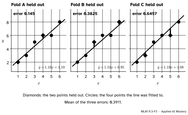
Three-fold cross-validation on six points, by hand. The points are the course’s four and two more, made up for this lesson: \(x = 1, \dots, 6\) and \(y = 2, 3, 5, 6, 6, 8\). A shuffle puts the points with \(x = 1\) and \(4\) in fold A, \(x = 3\) and \(6\) in fold B, and \(x = 2\) and \(5\) in fold C. Two candidates compete: a straight line fitted by least squares, and the flat line at the mean of the training targets (ridge with an endless price).
Fold A held out. The training points are \((2, 3)\), \((3, 5)\), \((5, 6)\) and \((6, 8)\), with \(\bar{x} = 4\) and \(\bar{y} = 5.5\). Their distances from the means are \(-2, -1, 1, 2\) in \(x\) and \(-2.5, -0.5, 0.5, 2.5\) in \(y\). As in lesson 1,
so \(w = 2.75/2.5 = 1.1\) and \(b = 5.5 - 1.1 \times 4 = 1.1\). Now score the two points that were held out. At \(x = 1\) the line says \(2.2\) and the target is \(2\): an error of \(0.2\). At \(x = 4\) it says \(5.5\) and the target is \(6\): an error of \(-0.5\).
The three rounds. Each line is fitted to the four circles and scored on the two diamonds by the purple bars.
The flat line. In fold A it answers \(5.5\) for both held-out points, which is wrong by \(3.5\) and by \(-0.5\): \(E_A = (12.25 + 0.25)/2 = 6.25\). Folds B and C give \(7.3125\) and \(2.8125\), so
The line wins easily. Its three fold errors differ more than fourfold, and a single split would have reported just one.
Code
A fold is a list of example numbers, and a “fitter” takes training data and returns a function that predicts.
import numpy as npdef kfold(n, k, seed): order = np.random.default_rng(seed).permutation(n) # shuffle the example numbers ...return np.array_split(order, k) # ... and cut the shuffled row into k foldsdef cross_validate(fitter, x, y, folds):"""The error of each fold: fit on the other folds, score on this one.""" errors = []for held_out in folds: rest = np.setdiff1d(np.arange(len(y)), held_out) # every example not in this fold predict = fitter(x[rest], y[rest]) errors.append(np.mean((predict(x[held_out]) - y[held_out]) **2))return np.array(errors)def fit_line(x, y): w = np.mean((x - x.mean()) * (y - y.mean())) / np.mean((x - x.mean()) **2)returnlambda q: w * q + y.mean() - w * x.mean()fit_mean =lambda x, y: (lambda q: np.full(len(q), y.mean()))x6 = np.array([1.0, 2.0, 3.0, 4.0, 5.0, 6.0])y6 = np.array([2.0, 3.0, 5.0, 6.0, 6.0, 8.0])folds6 = [np.array([0, 3]), np.array([2, 5]), np.array([1, 4])] # A, B, C as positions in the arraysfor name, fitter in [("line", fit_line), ("mean", fit_mean)]: errors = cross_validate(fitter, x6, y6, folds6)print(f"{name}: fold errors {np.round(errors, 4)}, cross-validation error {errors.mean():.4f}")
Now the real question: which price for the degree-9 polynomial? The 24 examples are the dozen and the twelve validation points of lesson 1, pooled. The standardising happens inside the fitter, so in every round it uses that round’s 18 training examples only.
x_train = (np.arange(12) +0.5) /12y_train = np.array([0.18, 1.06, 0.84, 0.67, 0.33, -0.02, -0.40, -1.11, -0.66, -1.37, -0.38, -0.40])x_val = np.array([0.11, 0.34, 0.36, 0.37, 0.43, 0.58, 0.60, 0.75, 0.85, 0.87, 0.91, 0.98])y_val = np.array([0.93, 0.76, 0.45, 1.03, 0.11, -0.21, -0.23, -1.20, -0.88, -1.14, -0.89, -0.45])x_pool, y_pool = np.concatenate([x_train, x_val]), np.concatenate([y_train, y_val])def powers(x, degree=9): u =2* x -1return np.column_stack([u ** k for k inrange(1, degree +1)])def fit_ridge(lam, degree=9):"""A fitter for ridge with price lam: standardise with the training part, solve, return a predictor."""def fitter(x, y): F = powers(x, degree) mu, sd = F.mean(axis=0), F.std(axis=0) Z, b, n = (F - mu) / sd, y.mean(), len(y) w = np.linalg.solve(Z.T @ Z / n + lam * np.eye(degree), Z.T @ (y - b) / n)returnlambda q: (powers(q, degree) - mu) / sd @ w + breturn fittergrid = np.array([m *10.0** e for e inrange(-6, 1) for m in (1, 3)] + [10.0]) # 1e-6, 3e-6, ..., 3, 10folds = kfold(24, 4, seed=2)table = np.array([cross_validate(fit_ridge(lam), x_pool, y_pool, folds) for lam in grid])for lam, errors inzip(grid, table):print(f"lam = {lam:<7g} fold errors {np.round(errors, 3)} mean {errors.mean():.3f}")best = grid[table.mean(axis=1).argmin()]final = fit_ridge(best)(x_pool, y_pool) # the winner, refitted to all 24print(f"chosen price: {best:g}. Fits: {table.size} for the search, plus 1 refit.")
lam = 1e-06   fold errors [ 0.137 17.074  0.872  0.072]  mean 4.539
lam = 3e-06   fold errors [ 0.132 12.007  0.431  0.071]  mean 3.160
lam = 1e-05   fold errors [0.123 6.581 0.176 0.071]  mean 1.738
lam = 3e-05   fold errors [0.111 3.233 0.188 0.071]  mean 0.900
lam = 0.0001  fold errors [0.099 1.563 0.242 0.069]  mean 0.493
lam = 0.0003  fold errors [0.092 0.866 0.242 0.065]  mean 0.316
lam = 0.001   fold errors [0.089 0.392 0.231 0.059]  mean 0.193
lam = 0.003   fold errors [0.09  0.109 0.231 0.052]  mean 0.121
lam = 0.01    fold errors [0.102 0.044 0.243 0.043]  mean 0.108
lam = 0.03    fold errors [0.129 0.16  0.301 0.045]  mean 0.159
lam = 0.1     fold errors [0.186 0.09  0.452 0.083]  mean 0.203
lam = 0.3     fold errors [0.285 0.072 0.567 0.182]  mean 0.277
lam = 1       fold errors [0.448 0.377 0.515 0.347]  mean 0.422
lam = 3       fold errors [0.587 0.388 0.443 0.487]  mean 0.476
lam = 10      fold errors [0.691 0.319 0.476 0.597]  mean 0.521
chosen price: 0.01.  Fits: 60 for the search, plus 1 refit.
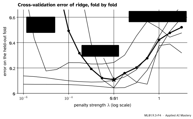
Cross-validation agrees with the single split of lesson 1 on \(\lambda = 0.01\), with a mean error of \(0.108\). At the tiny prices the mean explodes, to \(4.5\) at \(\lambda = 10^{-6}\): whenever an end point is held out, a barely penalised polynomial shoots off beyond its data.
ML01.9.3-F4
The four fold errors (thin) and their mean (thick) at each of the fifteen prices. The folds disagree with each other. Their mean still has a clear lowest point.
The experiment of the second figure: reshuffle a thousand times, recording the error of the first fold alone (a single split) and the mean of all four.
rng = np.random.default_rng(0)single, four = [], []for _ inrange(1000): errors = cross_validate(fit_ridge(0.01), x_pool, y_pool, np.array_split(rng.permutation(24), 4)) single.append(errors[0]) four.append(errors.mean())for name, values in [("one split", single), ("4-fold ", four)]: q1, q2, q3 = np.percentile(values, [25, 50, 75])print(f"{name}: middle half from {q1:.3f} to {q3:.3f}, median {q2:.3f}")
one split: middle half from 0.063 to 0.155, median 0.105
4-fold   : middle half from 0.100 to 0.126, median 0.110
The library version. KFold makes the folds, cross_val_score runs the rounds, and a Pipeline keeps the scaler inside them. Two details: scikit-learn scores are “higher is better”, so it reports the negative mean squared error, and Ridge’s alpha is \(n\lambda\) with \(n = 18\), the size of each round’s training set.
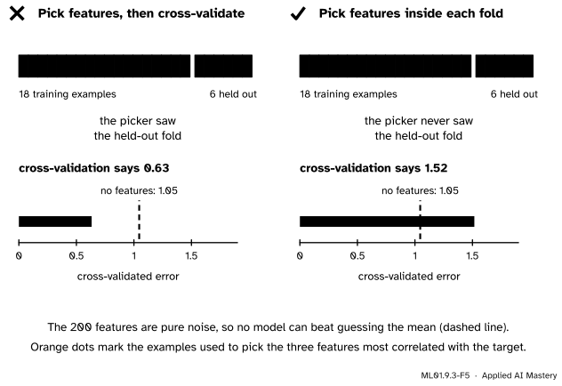
One last experiment, for the pitfalls below. The target and all 200 features are random numbers, so nothing can be predicted. A recipe picks the three features most correlated with the target and fits least squares to them. It is cross-validated twice: picking once on all 24 examples, and picking inside each round.
def pick(X, y, keep=3):"""The columns of X that are most strongly correlated with y.""" strength = np.abs((X - X.mean(axis=0)).T @ (y - y.mean())) / X.std(axis=0)return np.argsort(-strength)[:keep]def held_out_error(X, y, rest, held_out, columns): A = np.column_stack([np.ones(len(rest)), X[rest][:, columns]]) coef = np.linalg.lstsq(A, y[rest], rcond=None)[0] guess = np.column_stack([np.ones(len(held_out)), X[held_out][:, columns]]) @ coefreturn np.mean((guess - y[held_out]) **2)rng = np.random.default_rng(0)outside, inside, no_features = [], [], []for _ inrange(200): X, y = rng.normal(size=(24, 200)), rng.normal(size=24) order = rng.permutation(24) picked_once = pick(X, y) # the leak: all 24 examples help to pick rounds = [(np.setdiff1d(order, held_out), held_out) for held_out in np.array_split(order, 4)] outside.append(np.mean([held_out_error(X, y, rest, held, picked_once) for rest, held in rounds])) inside.append(np.mean([held_out_error(X, y, rest, held, pick(X[rest], y[rest])) for rest, held in rounds])) no_features.append(np.mean([np.mean((y[rest].mean() - y[held]) **2) for rest, held in rounds]))print(f"picked outside the folds: {np.mean(outside):.2f} picked inside: {np.mean(inside):.2f} "f"no features at all: {np.mean(no_features):.2f}")
picked outside the folds: 0.63 picked inside: 1.52 no features at all: 1.05
Explore
The module’s interactive, the penalty explorer, is in lesson 2. Its U-shaped curve comes from one fixed validation set of twelve points. Slide to \(\lambda = 0.01\) and compare its \(0.126\) with the four fold errors above: that is how far such a curve can move when the jury changes.
Pitfalls
ML01.9.3-F5
Wrong beside right, on targets and 200 features that are all pure noise. Left: picking the three “best” features with every example and then cross-validating reports \(0.63\), as if the noise could be predicted. Right: picking inside each round reports \(1.52\), worse than using no features, which is the truth.
“Prepare the data once, then cross-validate the model.”
Any step that learns from the examples is part of the model and belongs inside the folds: scaling, picking features, choosing a price. Run once on all the data, it has already seen the held-out fold. With a scaler the leak is usually small (ML01.2.4). With feature picking it is ruinous: \(0.63\) against an honest \(1.52\). In scikit-learn, put the steps in a Pipeline.
“The winner’s cross-validation error is the number to report.”
It was used to choose the winner, so it is spent, like a validation error (ML01.2.2, Result 2). An honest report needs a test set that is kept out of the cross-validation altogether. The next lesson is about that.
“KFold shuffles for me.”
Not by default: KFold(n_splits=4) cuts the rows as they stand. Sort the 24 examples by \(x\) and the folds become four stretches of the input range, so each model is tested on a region it never saw. The cross-validation error at \(\lambda = 0.01\) is then \(1.18\) instead of \(0.11\). Pass shuffle=True and a random_state, unless the order carries meaning, as time does.
“Cross-validation gives me a trained model.”
It gives a score for a recipe. The \(k\) models it fitted are by-products. Refit the chosen recipe on all the examples.
Check yourself
Recall
1. In one round of k-fold cross-validation, which examples fit the model and which score it?
Show answer
The examples of \(k - 1\) folds fit it. The one fold held out scores it.
2. What is the cross-validation error?
Show answer
The mean of the \(k\) fold errors. With equal folds it is the mean squared error over all \(n\) examples, each predicted by a model that never saw it.
3. How many fits does it take to choose among \(M\) candidates with \(k\) folds?
Show answer
\(kM\), plus one to refit the winner on all the data.
4. Name two ways in which cross-validation uses the data better than one split into equal training and validation halves.
Show answer
Each model is fitted to more examples, \((k - 1)/k\) of them instead of half. Every example takes part in judging, so the estimate rests on \(n\) scores instead of \(n/2\) and depends less on one lucky or unlucky draw.
5. Where must a scaler or a feature picker be fitted during cross-validation?
Show answer
Inside each round, on that round’s training folds only.
Exercises
1.★ You have 60 examples and 8 candidate prices, and use 5 folds. How large is each fold? On how many examples is each model fitted? How many fits are needed in all, counting the final one?
Show solution
Each fold has \(60/5 = 12\) examples. Each model is fitted on the other four folds, \(60 \times 4/5 = 48\) examples. The search takes \(5 \times 8 = 40\) fits and the refit of the winner one more: \(41\).
2.★★ Cross-validate ridge with \(\lambda = 0.25\) on the six points, with the folds of the worked example. The training statistics are: fold A, \(\bar{x} = 4\), \(\bar{y} = 5.5\), \(s_{xx} = 2.5\), \(s_{xy} = 2.75\); fold B, \(\bar{x} = 3\), \(\bar{y} = 4.25\), \(s_{xx} = 2.5\), \(s_{xy} = 2.75\); fold C, \(\bar{x} = 3.5\), \(\bar{y} = 5.25\), \(s_{xx} = 3.25\), \(s_{xy} = 3.875\). Does the penalty help?
Show solution
Use \(w = s_{xy}/(s_{xx} + \lambda)\) and \(b = \bar{y} - w\bar{x}\) in each fold.
Fold A: \(w = 2.75/2.75 = 1\), \(b = 5.5 - 4 = 1.5\). At \(x = 1\) and \(4\) the line says \(2.5\) and \(5.5\), off by \(0.5\) and \(-0.5\): \(E_A = 0.25\).
Fold B: \(w = 1\), \(b = 4.25 - 3 = 1.25\). At \(x = 3\) and \(6\) it says \(4.25\) and \(7.25\), off by \(-0.75\) twice: \(E_B = 0.5625\).
Fold C: \(w = 3.875/3.5 = 1.107\), \(b = 5.25 - 1.107 \times 3.5 = 1.375\). At \(x = 2\) and \(5\) it says \(3.589\) and \(6.911\), off by \(0.589\) and \(0.911\): \(E_C = (0.347 + 0.829)/2 = 0.588\).
\(\text{CV} = (0.25 + 0.5625 + 0.588)/3 = 0.467\), above the \(0.391\) of the plain line. The penalty does not help: a straight line through six points has little freedom to overfit.
3.★★★ For the model “answer with the mean of the training targets”, derive the leave-one-out cross-validation error in terms of \(s_{yy}\), and evaluate it for the six points.
Show solution
Leave out example \(i\). The other targets sum to \(n\bar{y} - y_i\), so their mean is \((n\bar{y} - y_i)/(n - 1)\). The error on the example left out is
For the six points \(\bar{y} = 5\), the deviations are \(-3, -2, 0, 1, 1, 3\) and \(s_{yy} = (9 + 4 + 0 + 1 + 1 + 9)/6 = 4\). So \(\text{CV} = (6/5)^2 \times 4 = 5.76\), a little above the three-fold value \(5.458\), and well above the training error \(4\) of the mean.
Summary card
Cross-validation gives every example one turn at judging and \(k - 1\) turns at fitting.
ML01.9.3-F1
Four rounds, four errors, one mean.
Recipe. Shuffle, cut into \(k\) folds, hold each out in turn, average the \(k\) errors.
Formula.\(\text{CV} = \frac{1}{k}\sum_j E_j\), and with equal folds a mean over all \(n\) examples.
Choose, then refit. Lowest CV wins; fit the winner again on all the data.
Cost.\(kM\) fits for \(M\) candidates, plus one.
By hand. Six points, three folds: line \(0.3911\), mean \(5.458\).
The 24 examples.\(\lambda = 0.01\) wins with \(0.108\); one split’s middle half is \(0.063\) to \(0.155\), four folds’ \(0.100\) to \(0.126\).
Rule. Whatever learns from data goes inside the folds.
Sources and next steps
Sources. Each was opened and checked against this lesson on 12 November 2026.
Trevor Hastie, Robert Tibshirani and Jerome Friedman, The Elements of Statistical Learning, 2nd edition (free PDF from the authors). Section 7.10.1 defines the cross-validation estimate as a mean over all \(N\) examples, each predicted with its own part removed (equation 7.48), names 5 and 10 as typical choices of \(K\) and \(K = N\) as leave-one-out, says the chosen model is then fitted to all the data, and explains with a learning curve (Figure 7.8) why training on part of the data can overestimate the error. Section 7.10.2, “The Wrong and Right Way to Do Cross-validation”, is the source of the feature-picking pitfall: there, with 50 samples and 5,000 noise predictors, the wrong way reports an error rate of 3% where the truth is 50%.
Tengyu Ma and Andrew Ng, CS229 Lecture Notes, Stanford University, Section 9.3. Describes hold-out, k-fold and leave-one-out cross-validation step by step, notes that a single hold-out set “wastes” part of the data, that k-fold needs each model to be trained \(k\) times, and that the selected model is retrained on the entire training set.
scikit-learn 1.9 User Guide, Section 3.1, Cross-validation: evaluating estimator performance. Describes k-fold cross-validation, says it “can be computationally expensive, but does not waste too much data”, that “a test set should still be held out for final evaluation”, and (Section 3.1.1) that preprocessing such as standardisation and feature selection should be learnt from a training set, which a Pipeline does under cross-validation.
scikit-learn 1.9 API reference, KFold. Splits into consecutive folds “without shuffling by default”; n_splits defaults to 5 and shuffle to False.
Next.ML01.9.4 Tuning without cheating adds the test set back, shows what peeking at it costs, and treats the number of training steps as one more price to tune.