Swap the squared weight in the penalty for its absolute value and weights do not just shrink: some become exactly zero. Derive the one-feature lasso solution, soft thresholding, case by case, and see in the picture of a diamond and a circle why ridge does not do the same.
Write the lasso loss and say how its penalty differs from the ridge penalty near zero.
Derive the one-feature lasso solution by cases and state it as soft thresholding.
Explain with the diamond and the circle why the lasso gives exact zeros and ridge does not.
Fit a lasso by coordinate descent in NumPy and reproduce it with scikit-learn’s Lasso.
In review. The maths and code on this page are checked by automated tests on every change, but an independent reader has not signed it off yet. Spot a mistake or a confusing step? Tell us.
The question
Ridge makes the nine weights of the polynomial small, but at the prices we try it deletes none. Change one symbol in the penalty, from \(w^2\) to \(\abs{w}\), and at a modest price five of the nine weights are exactly zero. The model has dropped five of its features by itself. Why should so small a change make the difference between small and gone?
From the last lesson
1. By what factor does ridge multiply the least-squares slope of one feature?
Show answer
By \(s_{xx}/(s_{xx} + \lambda)\). It is below 1 and never 0.
2. Why is each feature standardised before a penalised fit?
Show answer
A weight’s size depends on its feature’s unit. After standardising, every feature has variance 1 and the price bears on all of them equally.
Intuition
The lasso charges for the size of each weight instead of its square:
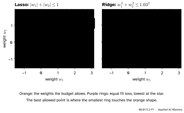
This is the L1 penalty. Picture two weights, \(w_1\) and \(w_2\), as a point in a plane. A penalty is the same as a budget: a region of the plane that the weights must stay inside (the formal section shows why). The fit loss is lowest at one point outside the region, and gets worse in rings around it. Training finds the point of the region on the smallest ring.
ML01.9.2-F1
The diamond and the circle. Both budgets cut \(w_1\) from \(2\) to \(1\). The lasso’s diamond is touched at a corner, where \(w_2\) is exactly \(0\). The ridge’s circle has no corners, and is touched where \(w_2 = 0.25\).
The diamond’s corners sit on the axes, where one weight is zero. A corner sticks out, so rings arriving from a whole wedge of directions hit it first. The circle is the same all the way round: with circular rings, as here, a ring touches it on an axis only if the star itself lies on that axis.
The same fact, told as prices: at a tiny weight ridge charges almost nothing for a little more, because the slope of \(w^2\) at zero is zero. The lasso charges the full rate \(\lambda\) per unit however small the weight is. If a feature’s first crumb of weight improves the fit by less than that, it is not worth buying at all.
Build it up
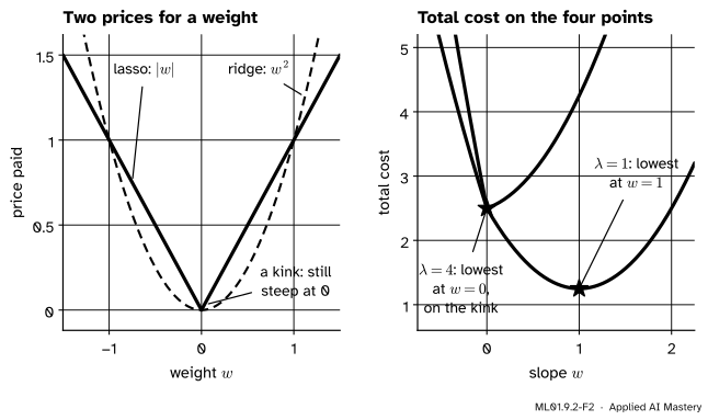
Step 1. Two prices. Plot what each penalty charges for one weight.
ML01.9.2-F2
Left: the ridge price is flat at zero; the lasso price has a kink there and is as steep as anywhere. Right: the fit loss of the four points plus the lasso price. At \(\lambda = 1\) the lowest point is at \(w = 1\). At \(\lambda = 4\) it is on the kink, at exactly \(w = 0\).
Step 2. One weight. For the course’s four points the fit loss is the parabola of lesson 1, lowest at \(w = 1.4\). Add \(\lambda\abs{w}\). The total is one parabola right of zero and another left of it, and they meet at \(w = 0\) in a kink.
Step 3. Where is the total lowest? For a low price, at the bottom of the right-hand parabola. For a high price that bottom would lie left of zero, where the right-hand parabola no longer applies. Then the lowest point is the kink itself: \(w = 0\) exactly.
Step 4. Subtract, do not divide. Ridge multiplies a weight by a factor below 1. The lasso subtracts a fixed amount and stops at zero.
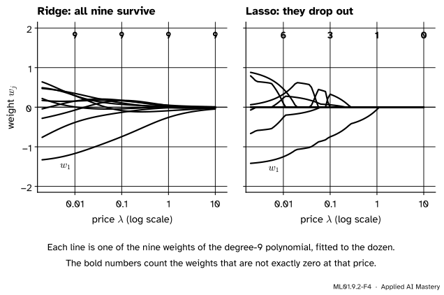
Step 5. Nine weights. On the degree-9 polynomial the features are correlated, so the weights no longer move one by one. But the pattern holds.
ML01.9.2-F4
The nine weights against the price. Left: ridge keeps all nine. Right: the lasso sets more of them to exactly zero as the price rises (a few leave zero for a while): three are left at \(\lambda = 0.1\), none at \(\lambda = 10\).
The formal statement
NoteDefinition: the lasso loss
For the model \(\hat{y}_i = w_1 x_{i1} + \dots + w_d x_{id} + b\) and a price \(\lambda \ge 0\),
Setting up. The penalty has no \(b\) in it, so Parts A and B of lesson 1 apply unchanged: the best bias is \(b = \bar{y} - w\bar{x}\), and with it the loss of the slope alone is
the loss falls all the way as \(w\) approaches \(0\) from the left. Downhill from both sides ends at \(w = 0\), and that is the minimum.
In Case 1 the same check shows that the left side slopes down towards \(0\), so the minimum found on the right is the lowest point overall. Case 2 is its mirror image.
In one line. Write \(S(a, \kappa)\) for “move \(a\) towards zero by \(\kappa\) (kappa), and stop at zero”: \(S(a, \kappa) = a - \kappa\) if \(a > \kappa\), \(a + \kappa\) if \(a < -\kappa\), and \(0\) otherwise. This is soft thresholding. Then
where \(w_{\text{ls}} = s_{xy}/s_{xx}\) is the least-squares slope. For a standardised feature, \(s_{zz} = 1\) and \(w_z = S(s_{zy}, \lambda/2)\). Compare ridge: \(w_z = s_{zy}/(1 + \lambda)\).
Two features that are not correlated. Let \(z_1\) and \(z_2\) be standardised, with \(\frac{1}{n}\sum_i z_{i1} z_{i2} = 0\), and write \(a_j = s_{z_j y}\). Expanding the square as in lesson 1, the fit loss \(F = \frac{1}{n}\sum_i (\hat{y}_i - y_i)^2\) is
No term mixes \(w_1\) with \(w_2\), and the penalty \(\lambda\abs{w_1} + \lambda\abs{w_2}\) does not mix them either. So each weight solves its own one-weight problem: \(w_j = S(a_j, \lambda/2)\). The fit loss is constant on circles around \((a_1, a_2)\): the rings of the anchor figure.
A penalty is a budget. Let \(\vect{w}^*\) minimise the fit loss plus \(\lambda P(\vect{w})\), where \(P\) is either penalty. Suppose some \(\vect{w}'\) with \(P(\vect{w}') \le P(\vect{w}^*)\) had a lower fit loss. Then its fit loss plus \(\lambda P(\vect{w}')\) would be lower than the total at \(\vect{w}^*\), which contradicts the choice of \(\vect{w}^*\). So among all weights that spend no more than \(P(\vect{w}^*)\), \(\vect{w}^*\) fits best. The weights that keep \(\abs{w_1} + \abs{w_2}\) within a budget form a diamond, and those that keep \(w_1^2 + w_2^2\) within one a disc.
Go deeper: correlated features: coordinate descent
When features are correlated, their mean product \(s_{12}\) is not \(0\), the term \(2w_1 w_2 s_{12}\) stays in \(F\), the rings become tilted ellipses and no formula gives all the weights at once. But hold every weight except \(w_j\) fixed, and what is left is a one-weight problem: fit feature \(j\) to the errors the other features leave behind. Its answer is the soft threshold. Coordinate descent applies this to each weight in turn, round after round, until nothing moves. The code below does exactly that, as does scikit-learn’s Lasso.
Frontier note: between the two penalties
The elastic net charges both prices at once, a mix of \(\abs{w}\) and \(w^2\). It keeps the lasso’s zeros and behaves better when features are strongly correlated, where the lasso picks one of a group almost at random.
Worked example
One weight: the four points. From lesson 1, \(s_{xx} = 1.25\), \(s_{xy} = 1.75\) and \(w_{\text{ls}} = 1.4\).
Price \(\lambda = 1\). Is \(s_{xy} > \lambda/2\)? Yes, \(1.75 > 0.5\): Case 1.
Price \(\lambda = 3.5\). Now \(\lambda/2 = 1.75 = s_{xy}\): Case 3, and \(w = 0\). From here on the model is the flat line \(\hat{y} = 4\).
Price \(\lambda = 4\). Still Case 3. Check it against the loss \(L(w) = 1.25w^2 - 3.5w + 2.5 + 4\abs{w}\): \(L(0) = 2.5\), \(L(0.1) = 2.5625\) and \(L(-0.1) = 3.2625\). Both neighbours are worse.
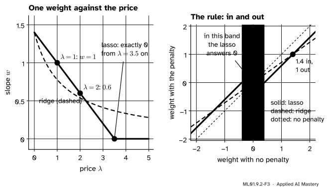
ML01.9.2-F3
Left: the lasso slope falls in a straight line and stops at zero; the ridge slope only creeps towards it. Right: the two rules for \(\lambda = 1\) (lasso) and \(\lambda = 0.5\) (ridge). Both send \(1.4\) to \(1\). Only the lasso has a band of inputs whose output is zero.
Two weights: four plots. A grower compares four plots of tomatoes (made up for this lesson). Feature 1 is fertiliser, low \({(-1)}\) or high \({(+1)}\). Feature 2 is extra watering, no \({(-1)}\) or yes \({(+1)}\). The yields are \(3, 3, 6, 8\) kg.
Plot
\(z_1\)
\(z_2\)
\(y\)
1
\(-1\)
\(-1\)
\(3\)
2
\(-1\)
\(+1\)
\(3\)
3
\(+1\)
\(-1\)
\(6\)
4
\(+1\)
\(+1\)
\(8\)
Each feature has mean \(0\) and variance \(1\), and their products \(+1, -1, -1, +1\) average \(0\): standardised and uncorrelated. The yields differ from their mean \(\bar{y} = 5\) by \(-2, -2, 1, 3\). Multiply these by each feature’s column and average:
So least squares says \(\hat{y} = 5 + 2z_1 + 0.5z_2\). Now charge each penalty.
\(w_1\)
\(w_2\)
Least squares
\(2\)
\(0.5\)
Lasso, \(\lambda = 2\): move each by \(1\)
\(2 - 1 = 1\)
\(0\), since \(0.5 \le 1\)
Ridge, \(\lambda = 1\): halve each
\(1\)
\(0.25\)
These are the two dots of the anchor figure: the lasso drops watering as not worth its price, while ridge keeps a quarter of a kilogram’s worth.
Code
import numpy as npdef soft(a, kappa):"""Move a towards zero by kappa, and stop at zero."""return np.sign(a) * np.maximum(np.abs(a) - kappa, 0.0)def lasso_line(x, y, lam): s_xx = np.mean((x - x.mean()) **2) s_xy = np.mean((x - x.mean()) * (y - y.mean())) w = soft(s_xy, lam /2) / s_xxreturnfloat(w), float(y.mean() - w * x.mean())x = np.array([1.0, 2.0, 3.0, 4.0])y = np.array([2.0, 3.0, 5.0, 6.0])for lam in [0.0, 1.0, 2.0, 3.5, 4.0]:print(f"lam = {lam}: w = {lasso_line(x, y, lam)[0]:.2f}, b = {lasso_line(x, y, lam)[1]:.2f}")L =lambda w: 1.25* w **2-3.5* w +2.5+4*abs(w)print("lam = 4, total loss at w = -0.1, 0, 0.1:", round(L(-0.1), 4), L(0.0), round(L(0.1), 4))
lam = 0.0: w = 1.40, b = 0.50
lam = 1.0: w = 1.00, b = 1.50
lam = 2.0: w = 0.60, b = 2.50
lam = 3.5: w = 0.00, b = 4.00
lam = 4.0: w = 0.00, b = 4.00
lam = 4, total loss at w = -0.1, 0, 0.1: 3.2625 2.5 2.5625
Now many weights, by the coordinate descent of the deeper block above.
def lasso_cd(Z, y, lam, sweeps=1000):"""Lasso by coordinate descent. Z holds standardised features, one per column.""" n, d = Z.shape w, b = np.zeros(d), y.mean()for _ inrange(sweeps):for j inrange(d): left_over = y - b - Z @ w + Z[:, j] * w[j] # errors with feature j taken out w[j] = soft(np.mean(Z[:, j] * left_over), lam /2) / np.mean(Z[:, j] **2)return w, bplots = np.array([[-1.0, -1.0], [-1.0, 1.0], [1.0, -1.0], [1.0, 1.0]])kg = np.array([3.0, 3.0, 6.0, 8.0])print("four plots, least squares:", lasso_cd(plots, kg, 0.0)[0])print("four plots, lasso lam = 2:", lasso_cd(plots, kg, 2.0)[0])print("four plots, ridge lam = 1:", np.linalg.solve(plots.T @ plots /4+ np.eye(2), plots.T @ (kg -5) /4))x_train = (np.arange(12) +0.5) /12# the dozen, as in lesson 1y_train = np.array([0.18, 1.06, 0.84, 0.67, 0.33, -0.02, -0.40, -1.11, -0.66, -1.37, -0.38, -0.40])x_val = np.array([0.11, 0.34, 0.36, 0.37, 0.43, 0.58, 0.60, 0.75, 0.85, 0.87, 0.91, 0.98])y_val = np.array([0.93, 0.76, 0.45, 1.03, 0.11, -0.21, -0.23, -1.20, -0.88, -1.14, -0.89, -0.45])def powers(x, degree=9): u =2* x -1return np.column_stack([u ** k for k inrange(1, degree +1)])F = powers(x_train)mu, sd = F.mean(axis=0), F.std(axis=0)Z, Z_val = (F - mu) / sd, (powers(x_val) - mu) / sdfor lam in [0.01, 0.03, 0.1]: w, b = lasso_cd(Z, y_train, lam)print(f"lam = {lam}: {np.sum(w !=0)} weights are not zero, training error "f"{np.mean((Z @ w + b - y_train) **2):.3f}, validation error {np.mean((Z_val @ w + b - y_val) **2):.3f}")w_lasso, b_lasso = lasso_cd(Z, y_train, 0.03)print("lam = 0.03:", np.round(w_lasso, 3) +0.0) # + 0.0 prints -0.0 as 0.0
four plots, least squares: [2.  0.5]
four plots, lasso lam = 2: [1. 0.]
four plots, ridge lam = 1: [1.   0.25]
lam = 0.01: 6 weights are not zero, training error 0.044, validation error 0.119
lam = 0.03: 4 weights are not zero, training error 0.055, validation error 0.114
lam = 0.1: 3 weights are not zero, training error 0.101, validation error 0.129
lam = 0.03: [-1.035  0.205  0.     0.     0.59   0.     0.    -0.127  0.   ]
At \(\lambda = 0.03\) five of the nine weights are exactly zero, not merely small: the model uses \(u\), \(u^2\), \(u^5\) and \(u^8\) only. Its validation error, \(0.114\), is a little below the best that ridge managed in lesson 1 (\(0.126\)).
The library version. scikit-learn’s Lasso puts a factor \(\frac{1}{2}\) in front of the mean squared error, so its alpha is \(\lambda/2\).
from sklearn.linear_model import Lasso, Ridgelibrary = Lasso(alpha=0.03/2, tol=1e-10, max_iter=100_000).fit(Z, y_train)print("scikit-learn, lam = 0.03:", np.round(library.coef_, 3) +0.0)z = (x - x.mean()) / x.std() # the four points, standardisedtwins = np.column_stack([z, z]) # the same feature, entered twiceprint("twins, lasso lam = 0.5:", np.round(Lasso(alpha=0.25).fit(twins, y).coef_, 3))print("twins, ridge lam = 0.5:", np.round(Ridge(alpha=4*0.5).fit(twins, y).coef_, 3))
The last two lines are a warning: given the same feature twice, ridge shares the weight, \(0.626\) each, and the lasso gives it all to the first copy.
Explore
ML01.9-X1
Penalty explorer
Slide the price from left to right and watch three things at once: the curve through the dozen, the nine weights, and the marker on the validation error. Then switch between L2 (ridge) and L1 (lasso) at the same price.
Under ridge, slide from far left to far right: no weight is ever exactly zero. Switch to the lasso at \(\lambda = 0.032\): four weights are left, as in the code above. Then press Lowest validation error under each penalty and compare the two prices. The bottom of the U is wide: many prices do nearly as well.
Pitfalls
ML01.9.2-F5
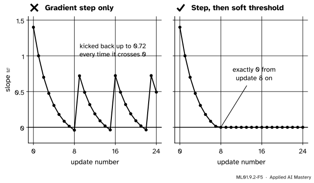
Wrong beside right, on the four points with \(\lambda = 4\), where the answer is \(w = 0\). Left: plain gradient steps on the lasso loss never settle. Right: a gradient step on the fit loss followed by a soft threshold lands on zero and stays.
“Train the lasso with ordinary gradient descent and the weights will hit zero.”
They will hover around it. The slope of \(\lambda\abs{w}\) jumps from \(-\lambda\) to \(+\lambda\) at zero, so a step that crosses zero is thrown back: here to \(0.72\), again and again. Exact zeros need an update that knows about the kink: a step on the fit loss, then the soft threshold \(S(\,\cdot\,, \eta\lambda)\).
“A zero weight means the feature is useless.”
It means the feature was not worth its price given the others. Of two identical features the lasso kept one and zeroed the other, though any split of the same total costs the same. Read a lasso’s zeros as “not needed alongside the rest”.
“Lasso(alpha=0.03) is our \(\lambda = 0.03\).”
scikit-learn’s lasso loss is \(\frac{1}{2n}\sum_i(\hat{y}_i - y_i)^2 + \alpha\sum_j\abs{w_j}\), half of ours when \(\alpha = \lambda/2\). So \(\lambda = 0.03\) is alpha=0.015. For Ridge the rule was different again: alpha\(= n\lambda\).
“The lasso always predicts better, because it removes noise features.”
Not always. Here it beat ridge by \(0.114\) to \(0.126\) on twelve validation points, a gap well inside the noise of so small a set. Which penalty is better is a question for validation data, like the price itself.
Check yourself
Recall
1. Write the lasso loss for a line \(\hat{y} = wx + b\).
Show answer
\(L = \frac{1}{n}\sum_i (wx_i + b - y_i)^2 + \lambda\abs{w}\).
2. What does soft thresholding \(S(a, \kappa)\) do?
Show answer
It moves \(a\) towards zero by \(\kappa\) and stops at zero: \(a - \kappa\) if \(a > \kappa\), \(a + \kappa\) if \(a < -\kappa\), and \(0\) in between.
3. For a standardised feature, give the ridge weight and the lasso weight in terms of \(s_{zy}\).
4. For which prices is the lasso weight of one feature exactly zero?
Show answer
For \(\lambda \ge 2\abs{s_{xy}}\). On the four points, from \(\lambda = 3.5\).
5. In the picture with two weights, why does the lasso solution often have a zero weight?
Show answer
Its budget region is a diamond whose corners lie on the axes. The smallest ring of equal fit loss often touches a corner first, and at a corner one weight is exactly zero.
Exercises
1.★ Fit the lasso to the four points with \(\lambda = 2.5\). Give the slope and the bias. Then give the ridge slope for the same price.
2.★★ Three standardised, uncorrelated features have least-squares weights \(3\), \(-1.2\) and \(0.4\). Find the lasso weights and the ridge weights for \(\lambda = 1\). From which price on is the second lasso weight zero?
Show solution
The features are uncorrelated, so each weight is handled alone and \(a_j\) is the least-squares weight. Lasso: move each towards zero by \(\lambda/2 = 0.5\), giving \(2.5\), \(-0.7\) and \(0\) (since \(0.4 \le 0.5\)). Ridge: divide each by \(1 + \lambda = 2\), giving \(1.5\), \(-0.6\) and \(0.2\). The second lasso weight is zero once \(\lambda/2 \ge 1.2\), that is from \(\lambda = 2.4\).
3.★★★ The elastic net for one centred feature minimises the loss below. Find its minimum, and check that it gives the lasso and ridge results as special cases.
This is the lasso loss of the formal section with \(s_{xx}\) replaced by \(s_{xx} + \lambda_2\) and \(\lambda\) by \(\lambda_1\), and the three cases never used anything about \(s_{xx}\) except that it is positive. So
\[
w = \frac{S(s_{xy},\ \lambda_1/2)}{s_{xx} + \lambda_2} .
\]
With \(\lambda_2 = 0\) this is the lasso result. With \(\lambda_1 = 0\) the threshold does nothing, \(S(s_{xy}, 0) = s_{xy}\), and \(w = s_{xy}/(s_{xx} + \lambda_2)\) is the ridge result. With both, the weight is first moved towards zero and then shrunk, and it is exactly zero whenever \(\lambda_1 \ge 2\abs{s_{xy}}\).
Summary card
The lasso charges for the size of a weight, not its square, and so it can set weights to exactly zero.
By hand. Four points: \(w = 1.4 - 0.4\lambda\) until it reaches \(0\) at \(\lambda = 3.5\).
The dozen.\(\lambda = 0.03\): four of nine weights left, validation error \(0.114\).
Library.Lasso(alpha=lam / 2).
Sources and next steps
Sources. Each was opened and checked against this lesson on 12 November 2026.
Trevor Hastie, Robert Tibshirani and Jerome Friedman, The Elements of Statistical Learning, 2nd edition (free PDF from the authors). Section 3.4.2 defines the lasso as a budget on \(\sum_j \abs{\beta_j}\) (equation 3.51) and as a penalty (3.52), and notes that there is no closed form in general and that a small enough budget makes some coefficients exactly zero. Section 3.4.3 gives, for orthonormal inputs, ridge as \(\hat\beta_j/(1 + \lambda)\) and the lasso as soft thresholding (Table 3.4), and draws the diamond and the disc (Figure 3.11): “Unlike the disk, the diamond has corners”. Section 3.8.6 describes coordinate descent with the soft-threshold update (3.84). Their lasso loss is \(\frac12\sum(\cdot)^2 + \lambda\sum\abs{\beta_j}\), so their threshold is \(\lambda\) where ours is \(\lambda/2\).
Ian Goodfellow, Yoshua Bengio and Aaron Courville, Deep Learning, MIT Press, 2016, Section 7.1.2. Gives the one-weight solution (equation 7.23): the unpenalised weight \(w_i^*\) is moved towards zero by \(\alpha/H_{i,i}\) and stopped at zero. It is ours with \(H = 2s_{xx}\) and \(\alpha = \lambda\).
scikit-learn 1.9 User Guide, Section 1.1.3, Lasso, gives the objective \(\frac{1}{2n}\norm{\mat{X}\vect{w} - \vect{y}}^2 + \alpha\norm{\vect{w}}_1\) and says that the lasso “is able to set coefficients exactly to zero”. Section 1.1.5 gives the elastic net, which mixes the two penalties.
Next.ML01.9.3 Cross-validation asks how far twelve validation points can be trusted to pick a price, and gives every example a turn at judging.