A yes-or-no prediction can be right in two ways and wrong in two ways. The confusion matrix counts all four. Learn to build it, read accuracy off its diagonal, and see why a model that never catches a single fraud can still be 99 percent accurate.
Name the four outcomes of a yes-or-no prediction and place each one in the confusion matrix.
Build a confusion matrix from labels and predictions, by hand and in NumPy.
Compute accuracy and the error rate from the four counts.
Explain, by writing accuracy as a weighted average of the two rows, why it misleads when one class is rare.
Compare a model’s accuracy with the accuracy of always predicting the larger class.
In review. The maths and code on this page are checked by automated tests on every change, but an independent reader has not signed it off yet. Spot a mistake or a confusing step? Tell us.
The question
A bank tests a model that checks card payments for fraud. On 1,000 payments it gives the right answer 990 times: 99% accuracy. Would you put it to work? Here is the catch: it has never flagged a single payment. How can a model that does nothing score 99%, and what should you look at instead of that one number?
Intuition
In lesson ML01.6.4 a model gave each of ten students a probability of passing. With the threshold \(0.5\) it called five of them a pass and five a fail, and it made two mistakes: one false alarm and one miss.
Every yes-or-no prediction ends in one of four ways. To name them, first choose a positive class: the answer you are looking for. Here it is “pass”. The other answer is the negative class.
A true positive (TP): the model says positive, and it is right.
A false positive (FP): the model says positive, and it is wrong. This is the false alarm.
A false negative (FN): the model says negative, and it is wrong. This is the miss.
A true negative (TN): the model says negative, and it is right.
The second word is what the model said. The first word says whether that was right.
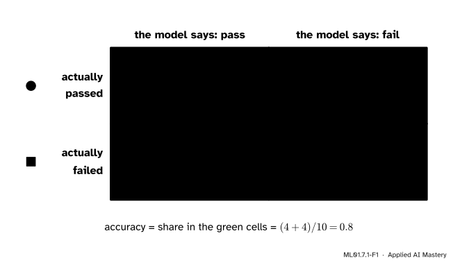
Count the students of each kind and set the four counts in a square. That table is the confusion matrix.
ML01.7.1-F1
The confusion matrix of the ten students at threshold \(0.5\). Each row is what was true, each column is what the model said. The correct answers sit on one diagonal, the mistakes on the other.
The simplest summary of the table is the accuracy: the share of the answers that are correct. Eight of the ten students are in the green cells, so the accuracy is \(0.8\).
Build it up
Step 1. Choose the positive class. “Positive” does not mean good. It means the thing the model is there to find: a pass, a fraud, an illness, a spam email. When one class is rare, it is nearly always the positive one.
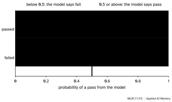
Step 2. The truth splits the examples, and the threshold splits them again. Line the students up by their probability, with those who passed in one row and those who failed in another. The threshold cuts both rows.
ML01.7.1-F2
The strip of probabilities from lesson ML01.6.4 is already a confusion matrix. Two rows for the truth, two sides of the cut for the model’s answer: four regions.
Step 3. Count each region. Four passes are right of the cut (TP) and one is left of it (FN). One fail is right of the cut (FP) and four are left of it (TN). In this course the matrix always has a row for each true class and a column for each answer of the model, positive class first:
Says pass
Says fail
Passed
TP \(= 4\)
FN \(= 1\)
Failed
FP \(= 1\)
TN \(= 4\)
Step 4. Accuracy and error rate. The correct answers are \({4 + 4 = 8}\) of \(10\), an accuracy of \(0.8\). The mistakes are \({1 + 1 = 2}\) of \(10\), an error rate of \(0.2\).
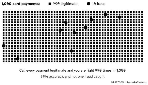
Step 5. Now make one class rare. Here are 1,000 card payments, invented for this module. Ten are fraud and 990 are legitimate. Fraud is the positive class.
ML01.7.1-F3
One payment in a hundred is fraud. A model can ignore the ten circles altogether and still be right about 990 marks.
Take the laziest model there is: it says “legitimate” every time. It is right about all 990 legitimate payments and wrong about the 10 frauds. Its accuracy is \({990 / 1000 = 0.99}\).
Step 6. So read an accuracy beside a baseline. Always answering with the larger class takes no skill, and its accuracy is the share of the larger class. Here that baseline accuracy is \(0.99\). An accuracy means something only when it is compared with this number, and even then it does not say which examples the model gets right.
A model gives one of two answers for each of \(n\) examples. Let TP, FN, FP and TN be the numbers of true positives, false negatives, false positives and true negatives. The confusion matrix is
Here \({n = \text{TP} + \text{FN} + \text{FP} + \text{TN}}\). The top row adds up to the number of actual positives, \({P = \text{TP} + \text{FN}}\). The bottom row adds up to the number of actual negatives, \({N = \text{FP} + \text{TN}}\). Three results follow.
Result 1: accuracy and error rate add up to 1. Every example is counted in exactly one cell, so
An accuracy of \(0.99\) and an error rate of \(0.01\) are the same statement.
Result 2: accuracy is a weighted average of the two rows. Let \({\rho = P / n}\) be the share of positives in the data, called the prevalence. Then \({N / n = 1 - \rho}\). Split the accuracy into its two terms, and multiply and divide each by its own row total:
\(\text{TP} / P\) is the share of the positives that the model finds. \(\text{TN} / N\) is the share of the negatives that it leaves alone. Accuracy mixes the two, and the weights are the sizes of the classes. With \({\rho = 0.01}\) the positives carry a weight of one hundredth. Find every fraud or none of them, and the accuracy moves by at most \(0.01\).
Result 3: the baseline. A model that always says “negative” has no positives of either kind, so \({\text{TP} = \text{FP} = 0}\), and then \({\text{FN} = P}\) and \({\text{TN} = N}\). Its accuracy is \({N / n = 1 - \rho}\). A model that always says “positive” has accuracy \({P / n = \rho}\), by the same argument. The better of these two do-nothing models has accuracy
A model that always gives the same answer finds all of one class and none of the other, so its balanced accuracy is \({\tfrac12 (1 + 0) = 0.5}\) whatever the prevalence is. When the two classes are the same size, balanced accuracy and accuracy are equal, because then \({\rho = 1 - \rho = \tfrac12}\) in Result 2. scikit-learn calls it balanced_accuracy_score. The next lesson gives \(\text{TP} / P\) its usual name, recall.
Worked example
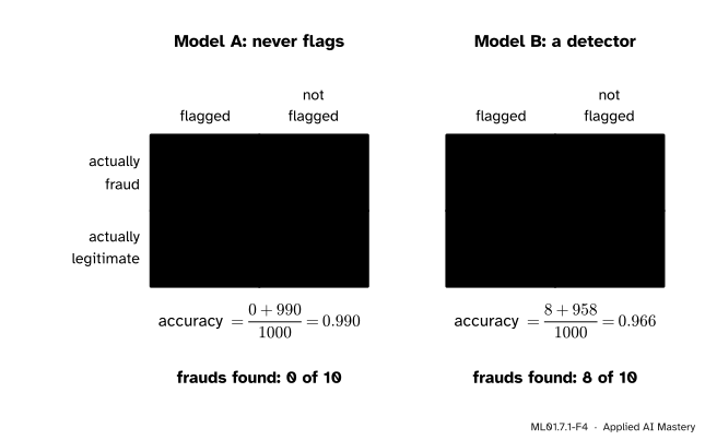
Two models for the 1,000 payments. Model A never flags a payment. Model B is a real detector: it flags 40 payments, and 8 of them are fraud.
Model A. Nothing is flagged, so \({\text{TP} = 0}\) and \({\text{FP} = 0}\). All 10 frauds are missed, \({\text{FN} = 10}\), and all 990 legitimate payments are left alone, \({\text{TN} = 990}\).
Model B. Of the 40 flagged payments, 8 are fraud: \({\text{TP} = 8}\), and the other \({40 - 8 = 32}\) are false alarms, \({\text{FP} = 32}\). Two frauds are not flagged: \({\text{FN} = 10 - 8 = 2}\). The legitimate payments left alone are \({\text{TN} = 990 - 32 = 958}\).
ML01.7.1-F4
The model that finds nothing has the higher accuracy. The matrices show why: almost all of both accuracies comes from the bottom-right cell.
Model A
Model B
Accuracy
\(\frac{0 + 990}{1000} = 0.990\)
\(\frac{8 + 958}{1000} = 0.966\)
Frauds found, \(\text{TP}/P\)
\(\frac{0}{10} = 0\)
\(\frac{8}{10} = 0.8\)
Legitimate left alone, \(\text{TN}/N\)
\(\frac{990}{990} = 1\)
\(\frac{958}{990} = 0.968\)
Check Result 2 on model B, with \({\rho = 10/1000 = 0.01}\):
Finding eight frauds in ten earned model B just \(0.008\) of accuracy. Its 32 false alarms cost it \({0.99 \times (1 - 0.968) = 0.032}\). So the useful model scores below the baseline of \(0.99\), and the useless one sits exactly on it. For this problem accuracy asks the wrong question. The next lesson asks better ones.
Code
From scratch: count the four outcomes, then divide.
import numpy as npdef confusion(y, said):"""The four counts (TP, FN, FP, TN), with 1 as the positive class.""" y, said = np.asarray(y), np.asarray(said) tp =int(np.sum((y ==1) & (said ==1))) fn =int(np.sum((y ==1) & (said ==0))) fp =int(np.sum((y ==0) & (said ==1))) tn =int(np.sum((y ==0) & (said ==0)))return tp, fn, fp, tndef accuracy(tp, fn, fp, tn):return (tp + tn) / (tp + fn + fp + tn)# The ten students of lesson ML01.6.4 and their model.study = np.array([1.0, 2.0, 2.0, 3.0, 4.0, 2.0, 3.0, 4.0, 4.0, 5.0])sleep = np.array([7.0, 5.0, 7.0, 5.0, 6.0, 6.0, 7.0, 5.0, 7.0, 5.0])passed = np.array([0, 0, 0, 0, 0, 1, 1, 1, 1, 1])p =1.0/ (1.0+ np.exp(-(study +0.5* sleep -6.0)))for threshold in [0.2, 0.5, 0.8]: counts = confusion(passed, (p >= threshold).astype(int))print(f"threshold {threshold}: (TP, FN, FP, TN) = {counts}, accuracy {accuracy(*counts):.1f}")
model A: (TP, FN, FP, TN) = (0, 10, 0, 990)  accuracy 0.990  found 0.0  left alone 1.000  weighted average 0.990
model B: (TP, FN, FP, TN) = (8, 2, 32, 958)  accuracy 0.966  found 0.8  left alone 0.968  weighted average 0.966
baseline accuracy: 0.99
The library version. Note the layout: scikit-learn sorts the classes, so class \(0\) comes first and the top-left cell is TN. Pass labels=[1, 0] to get the layout of this lesson.
Last, real data. scikit-learn’s digits dataset has 1,797 small images of handwritten digits, each 8 by 8 pixels, so 64 features. Ask one yes-or-no question of it: is this digit an 8? About one image in ten is, so the classes are imbalanced. A logistic regression is compared with DummyClassifier, which always predicts the most frequent class.
images: (1797, 64)  eights: 174
test images: 450  eights among them: 44
always 'not an 8': accuracy 0.902
logistic regression: accuracy 0.964
[[ 32  12]
 [  4 402]]
The detector of eights is \(96.4\%\) accurate on the 450 test images. That sounds excellent until it stands beside the \(90.2\%\) of a model that never says “eight”. And the matrix shows what the accuracy hides: of the 44 eights in the test set, the model finds 32 and misses 12.
Explore
This module’s interactive, the threshold slider, is in lesson 3. Press Very rare (1 : 99), so that one example in a hundred is positive, and drag the threshold all the way to the right. The model flags nothing, and the read-out shows an accuracy of \(0.99\). Now slide the threshold back to \(0.8\). The model finds 41 of the 100 positives without one false alarm, and the accuracy is still \(0.99\).
Pitfalls
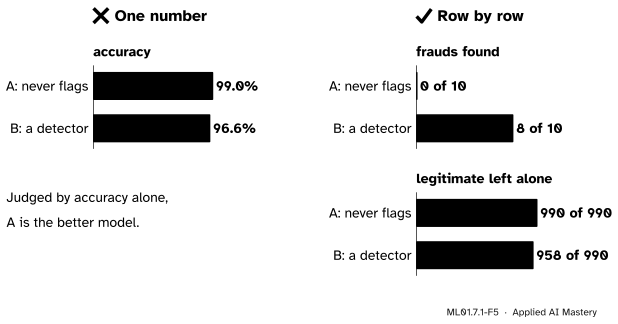
ML01.7.1-F5
Wrong beside right. One number ranks the do-nothing model first. Two numbers, one for each row of the matrix, show that it finds no fraud at all.
“99% accuracy: the model must be good.”
Not until you know the baseline. If 99% of the examples are negative, saying “negative” every time scores 99% as well. Report the accuracy of always predicting the larger class beside the model’s, and look at each row of the confusion matrix on its own.
“A false positive is a positive example.”
It is a negative example that the model called positive. In each name the second word is the model’s answer and the first word judges it. So the actual positives are the true positives plus the false negatives, \({P = \text{TP} + \text{FN}}\).
“The top-left cell is always the true positives.”
That depends on who drew the table. scikit-learn puts class \(0\) first, so its top-left cell holds the true negatives. Some books put the model’s answers in the rows and the truth in the columns. Read the row and column labels before you read a number.
“So accuracy is useless.”
No. When the classes are about the same size and the two mistakes cost about the same, as for the ten students, accuracy is a fair and simple summary. It fails when one class is rare or one mistake is much worse than the other, and many real problems are like that.
Check yourself
Recall
1. Name the four outcomes of a yes-or-no prediction.
Show answer
True positive, false positive, false negative and true negative.
2. In “false negative”, what does each word tell you?
Show answer
“Negative” is what the model said. “False” says that the answer was wrong. So the example was actually positive: a miss.
3. Write the accuracy in terms of the four counts.
4. What is the accuracy of a model that always predicts the larger class?
Show answer
The share of the larger class, \({\max(\rho, 1 - \rho)}\), where \(\rho\) is the share of positives.
5. Why does accuracy say so little about the positives when they are rare?
Show answer
Accuracy is \(\rho\) times the share of positives found, plus \({1 - \rho}\) times the share of negatives left alone. With a small \(\rho\) the first term can hardly move the total.
Exercises
1.★ A spam filter is tested on 200 emails, of which 50 are spam. It marks 60 emails as spam, and 45 of those really are spam. Build the confusion matrix, with spam as the positive class. Find the accuracy and the baseline accuracy.
Show solution
\({\text{TP} = 45}\). The other marked emails are false positives: \({\text{FP} = 60 - 45 = 15}\). The spam that was not marked: \({\text{FN} = 50 - 45 = 5}\). The rest of the 150 good emails: \({\text{TN} = 150 - 15 = 135}\).
Accuracy \({= (45 + 135)/200 = 0.9}\). The larger class is “not spam”, with 150 of 200 emails, so the baseline accuracy is \(0.75\). The filter is well above it.
2.★★ For the ten students, build the confusion matrix at threshold \(0.2\) and at threshold \(0.8\), and compute both accuracies. The probabilities are 0.182, 0.182, 0.378, 0.378 and 0.731 for the five fails, and 0.269, 0.622, 0.622, 0.818 and 0.818 for the five passes. What does the result say about accuracy?
Show solution
Threshold \(0.2\). Everyone except the two students at \(0.182\) is called a pass. All five passes are found: \({\text{TP} = 5}\), \({\text{FN} = 0}\). Three fails are called a pass: \({\text{FP} = 3}\), \({\text{TN} = 2}\). Accuracy \({= (5 + 2)/10 = 0.7}\).
Threshold \(0.8\). Only the two students at \(0.818\) are called a pass. \({\text{TP} = 2}\), \({\text{FN} = 3}\), \({\text{FP} = 0}\), \({\text{TN} = 5}\). Accuracy \({= (2 + 5)/10 = 0.7}\).
The two accuracies are equal, yet the mistakes are opposite: three false alarms and no miss, or three misses and no false alarm. Accuracy counts mistakes without saying which kind they are.
3.★★★ A detector finds a share \(a\) of the positives, more than none, and leaves alone a share \(b\) of the negatives. (a) Use Result 2 to show that its accuracy beats the “always negative” baseline exactly when \({\frac{\rho}{1 - \rho} > \frac{1 - b}{a}}\). (b) Model B has \({a = 0.8}\) and \({b = 958/990}\). How common must fraud be before model B beats the baseline on accuracy?
Show solution
(a) By Result 2 the accuracy is \({\rho a + (1 - \rho) b}\). The baseline is \({1 - \rho}\). So the detector wins when
\[
\begin{aligned}
&\rho a + (1 - \rho)\, b > 1 - \rho \\
&\rho a > (1 - \rho)(1 - b) \\
&\frac{\rho}{1 - \rho} > \frac{1 - b}{a} .
\end{aligned}
\]
The second line subtracts \({(1 - \rho)\, b}\) from both sides and takes out the common factor \({1 - \rho}\) on the right. The third divides by \(a\) and by \({1 - \rho}\), which are both positive.
(b) \({1 - b = 32/990 = 0.0323}\), so the right-hand side is \({0.0323 / 0.8 = 0.0404}\). Solving \({\frac{\rho}{1 - \rho} = 0.0404}\) gives \({\rho = 0.0404 / 1.0404 = 0.0388}\). Model B beats the baseline on accuracy only when more than about \(3.9\%\) of payments are fraud. At \(1\%\) it loses, although it has not changed at all. The comparison depends on the prevalence, not only on the model.
Summary card
Four outcomes, one table. Accuracy reads only its diagonal.
ML01.7.1-F1
Truth in rows, answers in columns.
Names. The second word is the model’s answer. The first word says whether it was right.
Baseline. Always predicting the larger class scores \({\max(\rho, 1 - \rho)}\).
1,000 payments, 10 fraud. Never flagging: accuracy \(0.990\), frauds found \(0\). A detector: \(0.966\) and \(8\) of \(10\).
Sources and next steps
Sources. Each was opened and checked against this lesson on 12 November 2026.
Daniel Jurafsky and James H. Martin, Speech and Language Processing, 3rd edition draft of 19 August 2026, Chapter 4, Section 4.9. Introduces the confusion matrix (Figure 4.7) and shows that a classifier which labels every one of a million tweets “not about pie”, when 100 of them are, has an accuracy of 99.99% and is useless.
Google, Machine Learning Crash Course, Thresholds and the confusion matrix. Defines the four outcomes with a spam example, and lays its table out with the truth in columns and the predictions in rows. The page Accuracy, recall, precision, and related metrics gives accuracy as \({(\text{TP} + \text{TN})}\) over all four counts and notes that a model which predicts negative every time scores 99% when one class appears 1% of the time.
Tom Fawcett, An introduction to ROC analysis, Pattern Recognition Letters 27 (2006), pages 861 to 874, Section 2. Defines the four outcomes and the two-by-two confusion matrix, and notes that the numbers along its major diagonal are the correct decisions. Read in the copy hosted by the University of Houston.
scikit-learn 1.9 User Guide, Metrics and scoring: Section 3.4.4.2 (accuracy score), Section 3.4.4.4 (balanced accuracy as the mean of the true positive and true negative rates), Section 3.4.4.6 (confusion matrix) and Section 3.4.8 (dummy estimators). The reference page for confusion_matrix states that entry \({i, j}\) counts the observations known to be in group \(i\) and predicted to be in group \(j\), so that in the binary case the true negatives are entry \({0, 0}\).
scikit-learn 1.9 documentation, load_digits: 1,797 samples, 64 features, 10 classes with about 180 samples each.
Next.ML01.7.2 Precision, recall and F1 reads the confusion matrix one row and one column at a time, which is what the rare class needs.