A probability becomes a decision when it is compared with a threshold. The border between the two answers is where the score is zero: a straight line in two features. Moving the threshold trades false alarms for misses, and softmax extends the model to many classes.
Find the decision boundary of a logistic regression model with one feature and with two.
Explain why the boundary is straight and why the weight vector is at a right angle to it.
Show how changing the threshold shifts the boundary, and count the false alarms and misses that result.
Compute softmax probabilities for three classes and show that two-class softmax is the sigmoid.
In review. The maths and code on this page are checked by automated tests on every change, but an independent reader has not signed it off yet. Spot a mistake or a confusing step? Tell us.
The question
A trained model says that a student has a 0.62 chance of passing. Is that a “pass”? And once the model looks at two things about each student, hours of study and hours of sleep, where on the map of study and sleep does “pass” end and “fail” begin? And what happens to the mistakes when you move that border?
From the last lesson
1. Write the two partial derivatives of the log loss of logistic regression.
2. What does scikit-learn’s LogisticRegression do by default that plain gradient descent on the log loss does not?
Show answer
It adds an L2 penalty on the weights, with strength set by \({C = 1}\). C=np.inf removes it.
Intuition
Logistic regression produces a probability. A decision needs one more ingredient, a threshold: answer “pass” when the probability is at least the threshold, and “fail” otherwise. The usual threshold is \(0.5\).
Since \({\sigma(0) = 0.5}\) and the sigmoid only ever rises, \({p \ge 0.5}\) happens exactly when the score \(z\) is at least \(0\). So the border between the two answers is the set of inputs whose score is zero. It is called the decision boundary.
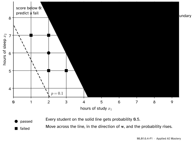
With one feature the boundary is a single point: for the six students it was \(3.5\) hours. To see more, give the model a second feature. Here are ten students, again invented for this module, with their hours of study \(x_1\) and their hours of sleep the night before, \(x_2\). The model is
\[
z = x_1 + 0.5\,x_2 - 6 , \qquad p = \sigma(z) .
\]
In this model one hour of study counts as much as two hours of sleep.
ML01.6.4-F1
The decision boundary of the model \({z = x_1 + 0.5\,x_2 - 6}\) is a straight line. Lines of equal probability run parallel to it, and the weight vector points straight across them, towards “pass”. One fail lies on the pass side and one pass on the fail side.
Build it up
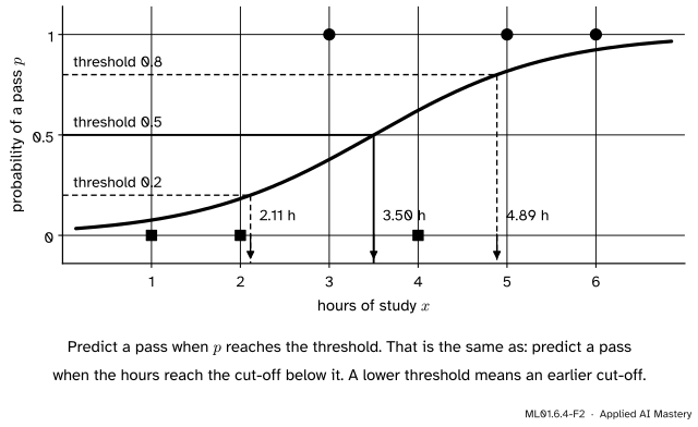
Step 1. One feature: a threshold on \(p\) is a cut-off on \(x\). Take the model \({p = {\sigma(x - 3.5)}}\) of lesson 1. With threshold \(0.5\), “predict a pass when \({p \ge 0.5}\)” is the rule “predict a pass when \({x \ge 3.5}\)”. Any other threshold is another cut-off, found by reading the curve backwards.
ML01.6.4-F2
Reading the curve backwards. A threshold of \(0.2\) puts the cut-off at \(2.11\) hours, a threshold of \(0.8\) at \(4.89\) hours.
Step 2. Two features: the boundary is a line. The score is zero where \({x_1 + 0.5\,x_2 - 6 = 0}\): a straight line through \({(2, 8)}\), \({(3, 6)}\) and \({(4, 4)}\). On one side the score is positive and the model says “pass”. On the other it is negative.
Step 3. The weights point across the boundary. Walk along the line, say one hour more study and two hours less sleep. The score changes by \({1 \cdot 1 + 0.5 \cdot (-2)} = 0\): nothing. Walk in the direction \({(1, 0.5)}\), the weights themselves, and the score rises as fast as it can. The weight vector is at a right angle to the boundary.
Step 4. Another threshold gives a parallel line. Every line “score \(=\) constant” is parallel to the boundary, and the probability is constant along it. So changing the threshold slides the boundary sideways without turning it.
Step 5. Two kinds of mistake. A false alarm is a predicted pass that was a fail. A miss is a predicted fail that was a pass. Lower the threshold and the model says “pass” more often: fewer misses, more false alarms. Raise it and the trade runs the other way. Module ML01.7 calls these mistakes false positives and false negatives.
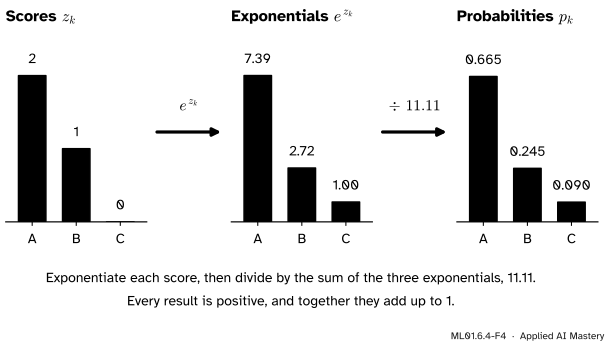
Step 6. More than two answers. Suppose the result is a grade, A, B or C. Give each grade its own score, a straight-line function of the inputs with its own weights. To turn three scores into three probabilities, make them positive by exponentiating, then divide by their sum so that they add up to \(1\). This is the softmax.
ML01.6.4-F4
Softmax in two moves, for the scores \({(2, 1, 0)}\). The largest score gets the largest probability, and the order of the three is kept.
The formal statement
NoteDefinition: decision rule and decision boundary
Given a model \({p = \sigma(z)}\) with score \(z = {\vect{w} \cdot \vect{x} + b}\) and a threshold \(\tau\) between \(0\) and \(1\), the decision rule is
The decision boundary is the set of inputs where \({p = \tau}\). For \({\tau = 0.5}\) it is the set where the score is zero, \({\vect{w} \cdot \vect{x} + b} = 0\).
Here \({\vect{w} \cdot \vect{x}} = w_1 x_1 + \dots + w_d x_d\) is the dot product.
Result 1: a threshold on the probability is a threshold on the score. The log-odds function \(\ln\frac{p}{1 - p}\) is increasing, so applying it to both sides of \({p \ge \tau}\) keeps the inequality:
\[
\begin{aligned}
p \ge \tau
&\iff \ln\frac{p}{1 - p} \ge \ln\frac{\tau}{1 - \tau} \\
&\iff z \ge c, \\
&\qquad\ \text{where } c = \ln\frac{\tau}{1 - \tau} .
\end{aligned}
\]
The last step uses lesson 1: the log-odds of \(p\) are the score. For \({\tau = 0.5}\) the cut on the score is \({c = \ln 1 = 0}\). For \({\tau = 0.8}\) it is \({\ln 4 = 1.386}\), and for \({\tau = 0.2}\) it is \(-1.386\). With one feature and \({w > 0}\), solving \({wx + b \ge c}\) for \(x\) gives the cut-off \({x \ge {(c - b) / w}}\).
Result 2: the boundary is flat, and all thresholds give parallel boundaries. The boundary for threshold \(\tau\) is \({\vect{w} \cdot \vect{x} + b} = c\). That is one linear equation: a point with one feature, a line with two, a plane with three. Changing \(\tau\) changes only the constant \(c\).
Result 3: the weight vector is at a right angle to the boundary. Take any two points \(\vect{u}\) and \(\vect{v}\) on the same boundary. Both satisfy its equation:
\[
\vect{w} \cdot \vect{u} + b = c \quad\text{and}\quad \vect{w} \cdot \vect{v} + b = c .
\]
Subtract the second from the first. The \(b\) and the \(c\) cancel, leaving \({\vect{w} \cdot (\vect{u} - \vect{v})} = 0\). The step \({\vect{u} - \vect{v}}\) lies along the boundary, and its dot product with \(\vect{w}\) is zero. A zero dot product means a right angle.
Softmax. For \(K\) classes with scores \({z_1, \dots, z_K}\),
Every \(p_k\) is positive, because exponentials are. They add up to \(1\), because each is divided by the same total. And a larger score always gets a larger probability, so the predicted class is the one with the largest score.
Two classes give back the sigmoid. With \({K = 2}\),
after dividing top and bottom by \(e^{z_1}\). Logistic regression is softmax with two classes, and its single score is the difference of the two class scores. The border between any two classes \(j\) and \(k\) is where \({z_j = z_k}\), which is again a linear equation: softmax boundaries are straight too.
Go deeper: choosing the threshold from the cost of each mistake
Suppose a false alarm costs \(a\) and a miss costs \(m\), and the model’s probability \(p\) can be trusted. Predicting “pass” is wrong with probability \({1 - p}\), at an expected cost of \({(1 - p)\,a}\). Predicting “fail” is wrong with probability \(p\), at an expected cost of \({p\,m}\). “Pass” is the cheaper choice when
\[
\begin{aligned}
&(1 - p)\,a \le p\,m \\
&\iff a \le p\,(a + m) \\
&\iff p \ge \frac{a}{a + m} .
\end{aligned}
\]
Equal costs give the threshold \(0.5\). If a miss is four times as costly as a false alarm, the threshold is \({\frac{1}{1 + 4} = 0.2}\): say “pass” even when it is fairly unlikely, because overlooking a pass is expensive.
Worked example
Ten students, one model, three thresholds. The model is \({z = x_1 + 0.5\,x_2 - 6}\). For the first student, \(z = {1 + 0.5 \cdot 7 - 6} = -1.5\) and \({p = {\sigma(-1.5)} = 0.182}\). The others follow in the same way.
\({(x_1, x_2)}\)
Result \(y\)
Score \(z\)
\(p = \sigma(z)\)
\({(1, 7)}\)
fail
\(-1.5\)
\(0.182\)
\({(2, 5)}\)
fail
\(-1.5\)
\(0.182\)
\({(2, 7)}\)
fail
\(-0.5\)
\(0.378\)
\({(3, 5)}\)
fail
\(-0.5\)
\(0.378\)
\({(4, 6)}\)
fail
\(1\)
\(0.731\)
\({(2, 6)}\)
pass
\(-1\)
\(0.269\)
\({(3, 7)}\)
pass
\(0.5\)
\(0.622\)
\({(4, 5)}\)
pass
\(0.5\)
\(0.622\)
\({(4, 7)}\)
pass
\(1.5\)
\(0.818\)
\({(5, 5)}\)
pass
\(1.5\)
\(0.818\)
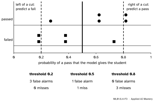
Threshold \(0.5\). One fail is above the threshold, the student at \({(4, 6)}\) with \({p = 0.731}\): a false alarm. One pass is below it, the student at \({(2, 6)}\) with \({p = 0.269}\): a miss.
Threshold \(0.2\). Everyone is predicted to pass except the two students at \(0.182\). No pass is overlooked, but three fails are above the threshold, at \(0.378\), \(0.378\) and \(0.731\).
Threshold \(0.8\). Only the two students at \(0.818\) are predicted to pass. No fail slips through, but three passes do, at \(0.269\), \(0.622\) and \(0.622\).
ML01.6.4-F3
The ten students lined up by their probability. A false alarm is a square to the right of the cut. A miss is a circle to the left of it. Sliding the cut to the left removes misses and adds false alarms.
Threshold
False alarms
Misses
\(0.2\)
3
0
\(0.5\)
1
1
\(0.8\)
0
3
No threshold removes both kinds of mistake, because one fail has a higher probability than one pass. The threshold only chooses which mistake to prefer. On the map, the three thresholds are parallel lines, where the score is \(-1.386\), \(0\) and \(1.386\).
Softmax by hand. For the grade scores \({(z_A, z_B, z_C)} = {(2, 1, 0)}\) the exponentials are \({e^{2} = 7.389}\), \({e^{1} = 2.718}\) and \({e^{0} = 1}\), and their sum is \(11.107\). So
The counts match the table. Next, the right angle and the one-feature cut-offs.
along = np.array([1.0, -2.0]) # a step along the boundaryprint("w . (step along the boundary) =", w @ along)for threshold in [0.2, 0.5, 0.8]: # one feature: p = sigmoid(x - 3.5)print(f"threshold {threshold}: cut-off at {np.log(threshold / (1- threshold)) +3.5:.2f} hours")
w . (step along the boundary) = 0.0
threshold 0.2: cut-off at 2.11 hours
threshold 0.5: cut-off at 3.50 hours
threshold 0.8: cut-off at 4.89 hours
Now train on the ten students, with the gradient of lesson 3 in its matrix form, on centred features.
def train(X, y, lr, steps): w, b = np.zeros(X.shape[1]), 0.0for _ inrange(steps): miss = sigmoid(X @ w + b) - y # p - y w, b = w - lr * X.T @ miss /len(y), b - lr * miss.mean()return w, bcentre = X.mean(axis=0) # (3, 6)w_fit, b_centred = train(X - centre, passed, lr=0.5, steps=1000)b_fit = b_centred - w_fit @ centre # the bias for the raw featuresprint("trained: w =", np.round(w_fit, 3), " b =", round(float(b_fit), 3))print("divided by w1:", np.round(w_fit / w_fit[0], 3), round(float(b_fit / w_fit[0]), 3))p_fit = sigmoid(X @ w_fit + b_fit)print("mistakes at 0.2, 0.5, 0.8:", [mistakes(p_fit, passed, t)[1:] for t in (0.2, 0.5, 0.8)])
trained: w = [1.214 0.607]  b = -7.282
divided by w1: [1.  0.5] -6.0
mistakes at 0.2, 0.5, 0.8: [(3, 0), (1, 1), (0, 3)]
Training finds \(\vect{w} = {(1.214,\ 0.607)}\), \({b = -7.282}\). Divided by \(w_1\), that is the hand model exactly: the same boundary, under a curve about \(1.2\) times steeper. (The ten students were placed so that this happens.)
The library version, with the penalty of lesson 3 switched off. predict uses the threshold \(0.5\), but it sends a score of exactly \(0\) to class \(0\), where our rule says \(1\). For any other threshold, compare the probabilities from predict_proba yourself.
from sklearn.linear_model import LogisticRegressionplain = LogisticRegression(C=np.inf).fit(X, passed) # no penaltyprint("scikit-learn: w =", np.round(plain.coef_[0], 2), " b =", round(float(plain.intercept_[0]), 2))proba = plain.predict_proba(X)[:, 1] # column 1 is the probability of class 1print("predict() equals (proba > 0.5):", np.array_equal(plain.predict(X), (proba >0.5).astype(int)))print("passes predicted at threshold 0.2:", int((proba >=0.2).sum()))
scikit-learn: w = [1.21 0.61]  b = -7.28
predict() equals (proba > 0.5): True
passes predicted at threshold 0.2: 8
The library agrees with our training.
Last, softmax: from scratch, from SciPy, and inside scikit-learn on iris, a real dataset that ships with it: 150 flowers with 4 measurements each, in 3 species of 50.
from scipy.special import softmax as scipy_softmaxfrom sklearn.datasets import load_irisdef softmax(scores): e = np.exp(scores - np.max(scores)) # subtracting a constant changes nothingreturn e / e.sum()print("softmax(2, 1, 0) =", np.round(softmax(np.array([2.0, 1.0, 0.0])), 3))print("softmax(z, 0)[0] =", round(float(softmax(np.array([1.5, 0.0]))[0]), 4), " sigmoid(z) =", round(float(sigmoid(1.5)), 4))iris = load_iris()model = LogisticRegression(max_iter=1000).fit(iris.data, iris.target)proba3 = model.predict_proba(iris.data)print("iris:", iris.data.shape, " probabilities for the first flower:", np.round(proba3[0], 3))print("every row sums to 1:", np.allclose(proba3.sum(axis=1), 1.0))print("correct on the training data:", int((model.predict(iris.data) == iris.target).sum()), "of 150")
softmax(2, 1, 0) = [0.665 0.245 0.09 ]
softmax(z, 0)[0] = 0.8176   sigmoid(z) = 0.8176
iris: (150, 4)  probabilities for the first flower: [0.982 0.018 0.   ]
every row sums to 1: True
correct on the training data: 146 of 150
The first two lines repeat the hand calculation and the two-class identity. The model gets 146 of the 150 flowers right, but on its own training data, which ML01.2 warned is not an honest estimate.
Explore
The sigmoid and boundary explorer is in lesson 3. Switch it to Two features: it opens on the map of this lesson. Slide the threshold to \(0.2\) and to \(0.8\). The boundary moves sideways without turning, and the read-out counts \(3\) false alarms and \(0\) misses, then \(0\) and \(3\). Then change \(w_2\) alone: the boundary turns, and the orange weight arrow stays at a right angle to it.
Pitfalls
ML01.6.4-F5
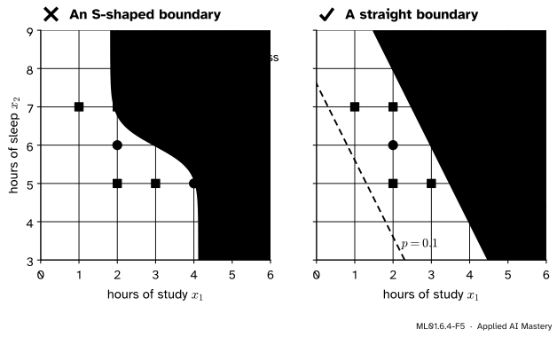
Wrong beside right. The S of the sigmoid is in the height of the probability as you walk across the boundary, not a shape on the map. There, the boundary and every line of equal probability are straight.
“The sigmoid is curved, so the decision boundary is curved.”
The boundary is where the score equals a constant, and the score is a straight-line function of the features. So the boundary is straight, whatever the weights are. Logistic regression cannot separate classes that need a bent border, such as one class surrounding the other. For that, give it new features such as \(x_1^2\) or \(x_1 x_2\), or use a different kind of model, like the nearest neighbours of ML01.3.
“The threshold is 0.5.”
That is a default. It treats the two mistakes as equally bad. When a miss is much worse than a false alarm, as in screening for an illness, a lower threshold is right. When a false alarm is worse, as in blocking a customer’s payment as fraud, a higher one is. Choose the threshold on validation data, from the costs.
“Changing the threshold changes the model.”
The threshold is applied after training. The weights, the probabilities and the log loss stay as they were. Only the decisions change, so one trained model can serve several uses that weigh the mistakes differently.
Check yourself
Recall
1. With threshold \(0.5\), where is the decision boundary of logistic regression?
Show answer
Where the score is zero: \({\vect{w} \cdot \vect{x} + b} = 0\). With one feature that is the point \({x = -b/w}\).
2. With two features, what shape is the boundary, and how is the weight vector related to it?
Show answer
A straight line. The weight vector is at a right angle to it and points towards the side where the model predicts \(1\).
3. What happens to the boundary when the threshold is raised from \(0.5\) to \(0.8\)?
Show answer
It moves, without turning, to where the score is \({\ln\frac{0.8}{0.2} = 1.386}\): towards the positive side, so fewer inputs are predicted to be \(1\).
4. You lower the threshold. Which kind of mistake becomes rarer, and which more common?
Show answer
Misses become rarer, because more examples are predicted positive. False alarms become more common.
5. Write the softmax. What does it reduce to for two classes?
Show answer
\(p_k = e^{z_k} / \sum_j e^{z_j}\). For two classes \({p_1 = {\sigma(z_1 - z_2)}}\), the sigmoid of the difference of the two scores.
Exercises
1.★ A model has score \({z = 2x_1 - x_2 - 1}\). Write its decision boundary as an equation for \(x_2\). Then give the probability and the decision at threshold \(0.5\) for the points \({(2, 1)}\), \({(1, 3)}\) and \({(1, 1)}\).
Show solution
The boundary is \({2x_1 - x_2 - 1 = 0}\), that is \({x_2 = 2x_1 - 1}\).
\({(1, 1)}\): \({z = 2 - 1 - 1 = 0}\), \({p = 0.5}\). The point is exactly on the boundary, and the rule “\({p \ge 0.5}\)” predicts \(1\).
2.★★ Use the table of the ten students. A miss costs four times as much as a false alarm. Compute the total cost at the thresholds \(0.2\), \(0.5\) and \(0.8\), counting a false alarm as \(1\). Which is cheapest, and does it agree with the formula in the “go deeper” note? Which other thresholds make exactly the same decisions as \(0.2\)?
Show solution
Cost \(=\) false alarms \({+\ 4 \times}\) misses. At \(0.2\): \({{3 + 4 \cdot 0} = 3}\). At \(0.5\): \({{1 + 4 \cdot 1} = 5}\). At \(0.8\): \({{0 + 4 \cdot 3} = 12}\). The threshold \(0.2\) is cheapest. The formula gives \(\frac{a}{a + m} = \frac{1}{1 + 4} = 0.2\), the same threshold.
No student has a probability between \({{\sigma(-1.5)} = 0.182}\) and \({{\sigma(-1)} = 0.269}\), so every threshold above the first and at most the second decides as \(0.2\) does.
3.★★★ Show that adding the same constant \(a\) to every score leaves the softmax probabilities unchanged. Use this to find the softmax of \({(3, 2, 1)}\) without new arithmetic, and to explain why two-class softmax needs only one score.
Show solution
Replace each \(z_k\) by \({z_k + a}\). Since \(e^{z_k + a} = e^{a}\,e^{z_k}\),
The factor \(e^{a}\) cancels, so the probabilities do not change. The scores \({(3, 2, 1)}\) are \({(2, 1, 0)}\) plus the constant \(1\), so their softmax is again \({(0.665,\ 0.245,\ 0.090)}\).
So only differences between scores matter. With two classes, subtract \(z_2\) from both: \({(z_1, z_2)}\) becomes \({(z_1 - z_2,\ 0)}\), with the same probabilities. One number, \({z = z_1 - z_2}\), carries everything, and \(p_1 = \frac{e^{z}}{e^{z} + 1} = \sigma(z)\). It is the single score of logistic regression.
Summary card
The boundary is where the score is zero, and it is straight.
ML01.6.4-F1
A straight border; weights point across it.
Decision rule. Predict \(1\) when \({p \ge \tau}\), which is when \(z \ge \ln\frac{\tau}{1 - \tau}\).
Boundary. For \({\tau = 0.5}\): \({\vect{w} \cdot \vect{x} + b} = 0\), with \(\vect{w}\) at a right angle to it. Other thresholds give parallel boundaries.
Trade-off. A lower threshold means fewer misses and more false alarms. Ten students: \({(3, 0)}\), \({(1, 1)}\), \({(0, 3)}\) at \(0.2\), \(0.5\), \(0.8\).
Sources. Each was opened and checked against this lesson on 12 November 2026.
Daniel Jurafsky and James H. Martin, Speech and Language Processing, 3rd edition draft of 19 August 2026, Chapter 4. Section 4.3 calls \(0.5\) the decision boundary. Section 4.7.1 defines the softmax (equation 4.33).
Google, Machine Learning Crash Course, Classification module, Thresholds and the confusion matrix. Says that \(0.5\) is not a good threshold when one kind of wrong classification costs more than the other, and that raising the threshold gives fewer false positives and more false negatives.
Aston Zhang, Zachary Lipton, Mu Li and Alexander Smola, Dive into Deep Learning, Section 4.1. Gives the softmax (equation 4.1.3) and notes in (4.1.4) that the most likely class has the largest score.
scikit-learn 1.9 documentation, LogisticRegression: predict_proba uses the softmax when there are more than two classes. Also load_iris: 150 samples, 4 features, 3 classes of 50.
Next. Module ML01.7, Evaluation metrics, builds the confusion matrix, precision, recall and the ROC curve from the false alarms and misses of this lesson.