A straight line is a poor model for a yes-or-no label: it predicts numbers below 0 and above 1. The sigmoid squashes any score into a probability, and the model that results is still a straight line, in the log-odds.
Explain two ways in which a straight line fails as a model of a yes-or-no label.
Compute the sigmoid of a score, and state its range, its midpoint and its symmetry.
Convert between a probability, the odds and the log-odds.
Show that logistic regression is linear in the log-odds, and read a weight as a multiplier of the odds.
In review. The maths and code on this page are checked by automated tests on every change, but an independent reader has not signed it off yet. Spot a mistake or a confusing step? Tell us.
The question
Six students studied for an exam, for one to six hours each. Three passed and three failed. You want a model that turns hours of study into the chance of passing. Fit a straight line and it tells you that seven hours of study gives a chance of 1.2, which is more than certain. What should replace the line?
Intuition
In regression (module ML01.4) the target is a quantity, and a line is a natural model. Here the target is an answer to a yes-or-no question. We write it as a label\(y\) that is \(1\) for yes and \(0\) for no. Predicting a label is called classification.
This module uses one tiny dataset, invented for the purpose: six students, the hours each studied in the week before an exam, and whether each passed.
Hours of study \(x\)
Passed? \(y\)
1
0
2
0
3
1
4
0
5
1
6
1
More study helps, but not reliably: the student with three hours passed and the one with four failed. So a good model should not answer “pass” or “fail” outright. It should give a probability of passing, a number between \(0\) and \(1\).
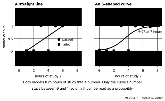
Nothing stops us from fitting a line to these six points, treating the labels as plain numbers. The least-squares line of ML01.4 comes out as \({\hat{y} = 0.2x - 0.2}\). Look at what it says.
ML01.6.1-F1
The same six students, two models. Left: the least-squares line gives \(-0.2\) for no study and \(1.2\) for seven hours. Neither is a probability. Right: an S-shaped curve does the same job and stays between \(0\) and \(1\) for every input.
The line is not a bad idea. It is an unfinished one. Keep the line, but stop calling its output a probability. Call it a score: any real number, where a higher score means “more likely to pass”. Then pass the score through a function that squashes the whole number line into the interval from \(0\) to \(1\). That function is the sigmoid, and a line followed by a sigmoid is logistic regression.
Build it up
Step 1. The line has a second fault: easy cases drag it around. Add a seventh student who studied 20 hours and passed. Nobody doubted that this student would pass, so the new example says nothing about where passing begins. Yet the least-squares line must tilt to reach it. The refitted line is \({\hat{y} = 0.042x + 0.325}\), and the point where it crosses \(0.5\) moves from \(3.5\) hours to \(4.16\) hours. A model of probabilities should not change its mind about borderline students because one certain case was added.
Step 2. The score. Write the line as
\[
z = w x + b ,
\]
with a weight\(w\) and a bias\(b\). Take \({w = 1}\) and \({b = -3.5}\) as an example, so \({z = x - 3.5}\). A student with five hours scores \(1.5\), and one with two hours scores \(-1.5\). A positive score leans towards a pass, a negative score towards a fail, and a score of \(0\) is undecided.
Step 3. The sigmoid squashes the score. The sigmoid is written \(\sigma\) (the Greek letter sigma):
\[
\sigma(z) = \frac{1}{1 + e^{-z}} .
\]
Read it from the inside. The number \(e^{-z}\) is always positive, so the denominator is always more than \(1\), and the fraction is always between \(0\) and \(1\). For a large positive score \(e^{-z}\) is tiny, and the fraction is just under \(1\). For a large negative score \(e^{-z}\) is huge, and the fraction is just over \(0\). At \({z = 0}\) we get \(\tfrac{1}{1 + 1} = \tfrac12\).
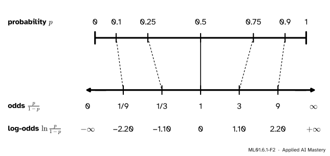
Step 4. Odds are a second way to state a probability. The odds of an event with probability \(p\) are \(\frac{p}{1 - p}\): how many times more likely it is to happen than not. A probability of \(0.75\) is odds of \({0.75 / 0.25 = 3}\), or “3 to 1”. A probability of \(0.5\) is odds of \(1\). Odds run from \(0\) up to infinity.
Step 5. Log-odds are a third way. Take the natural logarithm of the odds and the scale opens up in the other direction too. The log-odds are \(0\) for a coin flip, positive when the event is more likely than not, and negative when it is less likely.
ML01.6.1-F2
One belief on three scales. The probability ruler ends at \(0\) and \(1\). The log-odds ruler has no ends. Equal steps along the log-odds ruler are equal multiplications of the odds: each step of \(1.10\) multiplies the odds by \(3\).
The log-odds scale is the one a line can live on, because it runs from \({-\infty}\) to \({+\infty}\) just as a line does. The next section shows that this is exactly what logistic regression does: its score \(z\)is the log-odds.
The formal statement
NoteDefinition: logistic regression with one feature
The model has two parameters, a weight \(\cparam{w}\) and a bias \(\cparam{b}\). For an input \(\cdata{x}\) it computes a score and then a probability:
The output \(\cmodel{p}\) is read as the probability that the label is \(1\) for this input, \({p(y = 1 \mid x)}\). The probability that the label is \(0\) is \({1 - p}\).
Three properties of the sigmoid carry the whole module. Each is derived in full.
Property 1: the output is always strictly between 0 and 1. For every real \(z\), \({e^{-z} > 0}\). So \({1 + e^{-z} > 1}\), and dividing \(1\) by a number greater than \(1\) gives a result below \(1\). The result is also positive, because numerator and denominator are both positive. Hence \({0 < \sigma(z) < 1}\). The curve comes as close to \(0\) and to \(1\) as you like, and never touches them.
Property 2: the curve is symmetric about its midpoint. At \({z = 0}\), \({\sigma(0) = \tfrac12}\). For any \(z\),
Logistic regression is a linear model of the log-odds. The straight line never left. It moved to the one scale on which a straight line makes sense.
What the weight means. Raise \(x\) by one unit. The log-odds rise by \(w\), so the odds are multiplied by a fixed factor:
\[
\begin{aligned}
\frac{\text{odds at } x + 1}{\text{odds at } x}
&= \frac{e^{w(x + 1) + b}}{e^{wx + b}} \\
&= e^{w(x+1) + b - wx - b} \\
&= e^{w} .
\end{aligned}
\]
With \({w = 1}\), every extra hour multiplies the odds of passing by \({e \approx 2.72}\), whatever the starting point.
Where the curve crosses one half.\({p = \tfrac12}\) exactly when \({z = 0}\), that is when \({wx + b = 0}\), so at \({x = -b / w}\). For \({w = 1}\), \({b = -3.5}\) that is \(3.5\) hours. A natural rule for turning the probability into a decision is to predict a pass when \({p \ge \tfrac12}\). Lesson 4 studies that rule and its alternatives.
Go deeper: why this S-curve and not another one
Many curves rise smoothly from \(0\) to \(1\). The sigmoid is the only one for which the log-odds are exactly the score. To see it, start from that requirement and solve for \(p\):
Dividing top and bottom by \(e^{z}\) gives \({p = \frac{1}{1 + e^{-z}}}\), the sigmoid. The function \({p \mapsto \ln\frac{p}{1-p}}\) is called the logit, and the sigmoid is its inverse, which is why scores are often called logits.
A different choice is possible. The probit model squashes the score with the cumulative distribution function of the standard normal distribution instead. Its curve has the same S shape, but its weights no longer multiply the odds by a fixed factor.
Frontier note: the sigmoid inside neural networks
A unit of a neural network computes a weighted sum of its inputs and passes it through a squashing function. With the sigmoid as that function, one unit is a logistic regression. Deep networks for yes-or-no questions still end in exactly this unit, and the scores they feed it are called logits for the reason given above. For questions with many possible answers, such as “which word comes next?”, the sigmoid is replaced by its many-class version, the softmax of lesson 4.
Worked example
The model \({w = 1}\), \({b = -3.5}\), applied to two students.
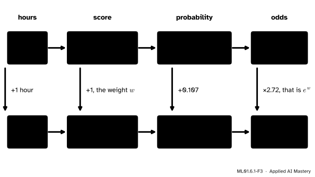
A student who studied 5 hours. The score is \(z = {1 \cdot 5 - 3.5} = 1.5\). Then \({e^{-1.5} = 0.2231}\), so
The odds are \(\frac{p}{1 - p} = e^{1.5} = 4.48\), and their logarithm is \(1.5\), the score we started from.
A student who studied 6 hours. The score is \(2.5\), so \({e^{-2.5} = 0.0821}\) and \(p = \frac{1}{1.0821} = 0.924\). The odds are \({e^{2.5} = 12.18}\).
ML01.6.1-F3
Two students through the model, column by column. One more hour adds \({w = 1}\) to the score, multiplies the odds by \({e^{w} = 2.72}\), and here adds \(0.107\) to the probability.
Compare the two. The extra hour added \(1\) to the score and multiplied the odds by \({12.18 / 4.48 = 2.72}\). The probability rose by \(0.107\). (Results are computed before rounding, which is why this is not \({0.924 - 0.818 = 0.106}\).)
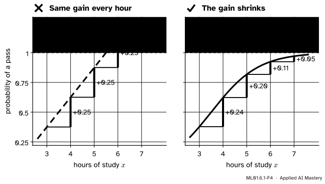
Now take the same extra hour earlier, from 3 hours to 4. The scores are \(-0.5\) and \(0.5\), the probabilities \(0.378\) and \(0.622\), and the odds \(0.607\) and \(1.649\). The odds are again multiplied by \(2.72\). The probability rises by \(0.245\), more than twice as much as before. One more hour is always the same step in log-odds, and a different step in probability.
For reference, here is the model’s answer for all six students. The symmetry of Property 2 shows in the last column: the entries add up to \(1\) in pairs from the outside in.
Hours \(x\)
Score \({z = x - 3.5}\)
Probability \({p = \sigma(z)}\)
1
\(-2.5\)
\(0.076\)
2
\(-1.5\)
\(0.182\)
3
\(-0.5\)
\(0.378\)
4
\(0.5\)
\(0.622\)
5
\(1.5\)
\(0.818\)
6
\(2.5\)
\(0.924\)
Code
From scratch first: the sigmoid is one line of plain Python.
import mathdef sigmoid(z):return1.0/ (1.0+ math.exp(-z))w, b =1.0, -3.5print(" x z p odds")for x inrange(1, 7): z = w * x + b p = sigmoid(z)print(f"{x:2d}{z:5.1f}{p:.3f}{p / (1- p):6.2f}")
 x      z      p    odds
 1   -2.5  0.076    0.08
 2   -1.5  0.182    0.22
 3   -0.5  0.378    0.61
 4    0.5  0.622    1.65
 5    1.5  0.818    4.48
 6    2.5  0.924   12.18
The table matches the worked example. Next, the straight line and its two faults, with NumPy.
import numpy as nphours = np.array([1.0, 2.0, 3.0, 4.0, 5.0, 6.0])passed = np.array([0.0, 0.0, 1.0, 0.0, 1.0, 1.0])slope, intercept = np.polyfit(hours, passed, 1) # the least-squares lineprint(f"line: y = {slope:.3f} x {intercept:+.3f}")print(f"at 0 hours: {intercept:.2f} at 7 hours: {slope *7+ intercept:.2f}")print(f"crosses 0.5 at {(0.5- intercept) / slope:.2f} hours")hours7, passed7 = np.append(hours, 20.0), np.append(passed, 1.0) # one more certain passslope7, intercept7 = np.polyfit(hours7, passed7, 1)print(f"with the 20-hour student: y = {slope7:.3f} x {intercept7:+.3f}")print(f"crosses 0.5 at {(0.5- intercept7) / slope7:.2f} hours")
line: y = 0.200 x -0.200
at 0 hours: -0.20   at 7 hours: 1.20
crosses 0.5 at 3.50 hours
with the 20-hour student: y = 0.042 x +0.325
crosses 0.5 at 4.16 hours
Last, the library version. SciPy calls the sigmoid expit and its inverse logit. Both work on whole arrays, and expit stays accurate for scores so extreme that the plain formula fails.
from scipy.special import expit, logitp = expit(w * hours + b)print("probabilities:", np.round(p, 3))print("log-odds: ", np.round(logit(p), 3))try: sigmoid(-800.0)exceptOverflowErroras error:print("plain formula at z = -800:", error)print("expit(-800) =", expit(-800.0))
probabilities: [0.076 0.182 0.378 0.622 0.818 0.924]
log-odds:      [-2.5 -1.5 -0.5  0.5  1.5  2.5]
plain formula at z = -800: math range error
expit(-800) = 0.0
The log-odds printed in the second row are the scores \({-2.5, \dots, 2.5}\): logit undoes expit, which is Property 3 in code. The last two lines show why libraries exist: \(e^{800}\) is too large for a floating-point number, so the one-line formula raises an error, while expit returns the correct answer, a probability too small to tell apart from \(0\).
Explore
The sigmoid and boundary explorer is in lesson 3. Its first two sliders are the \(w\) and \(b\) of this lesson, and it opens on the curve of the worked example, \({w = 1}\) and \({b = -3.5}\). Raise \(w\) to make the curve steeper, and change \(b\) to slide it sideways.
Pitfalls
ML01.6.1-F4
Wrong beside right, for the model \({w = 1}\), \({b = -3.5}\). Left: treating the curve’s steepest slope, \(0.25\) per hour, as the gain for everyone. Right: the real gains, read off the curve.
“Each extra hour adds the same amount of probability.”
That is the straight-line habit. In logistic regression each extra hour adds the same amount to the log-odds and multiplies the odds by the same factor \(e^{w}\). The gain in probability is largest near \({p = 0.5}\) and shrinks towards the ends, as on the right of the figure. A student who is almost sure to pass has little left to gain.
“Odds of 3 means a probability of 3, or of one third.”
Odds and probability are different scales. Odds of \(3\) mean \({{p / (1 - p)} = 3}\), so \({p = 0.75}\). Doubling the odds does not double the probability either: from odds \(1\) (\({p = 0.5}\)) to odds \(2\) is \({p = 0.667}\), not \({p = 1}\).
“The model outputs the answer, pass or fail.”
It outputs a probability. Turning \(0.62\) into “pass” is a separate decision that needs a threshold, and the right threshold depends on what each kind of mistake costs. Keep the probability for as long as you can: it says how sure the model is, which a bare label throws away.
“It is called regression, so it predicts a quantity.”
The name is historical. The model regresses the log-odds on the input, but it is used for classification.
Check yourself
Recall
1. Give two reasons why a least-squares line is a poor model of a yes-or-no label.
Show answer
Its outputs go below \(0\) and above \(1\), so they are not probabilities. And examples far from the boundary, which any model gets right, still tilt the line and move its crossing of \(0.5\).
2. Write the sigmoid function. What are \(\sigma(0)\) and the range of \(\sigma\)?
Show answer
\(\sigma(z) = \frac{1}{1 + e^{-z}}\). \({\sigma(0) = \tfrac12}\), and \({0 < \sigma(z) < 1}\) for every \(z\).
3. What are the odds and the log-odds of an event with probability \(0.75\)?
4. In logistic regression, which quantity is a straight-line function of the input \(x\)?
Show answer
The log-odds: \(\ln\frac{p}{1 - p} = wx + b\). The probability itself follows an S-shaped curve.
5. With weight \(w\), what does one more unit of \(x\) do to the odds?
Show answer
It multiplies them by \(e^{w}\). For \({w = 1}\) that is a factor of about \(2.72\).
Exercises
1.★ A model has \({w = 0.8}\) and \({b = -2}\). For \({x = 4}\), compute the score, the probability and the odds. At which \(x\) is the probability exactly \(0.5\)?
Show solution
Score: \(z = {0.8 \cdot 4 - 2} = 1.2\). Then \({e^{-1.2} = 0.3012}\), so \(p = \frac{1}{1.3012} = 0.769\). Odds: \({e^{1.2} = 3.32}\) (check: \({0.7685 / 0.2315 = 3.32}\)). The probability is \(0.5\) where \({z = 0}\): \({0.8x - 2 = 0}\), so \({x = 2.5}\).
2.★★ A model gives a student odds of 3 to 1 of passing, and its weight is \({w = 0.5}\) per hour of study. (a) What is the probability of passing? (b) What are the odds and the probability after two more hours? (c) How many extra hours would raise the odds from \(3\) to \(30\)?
Show solution
(a) \(p = \frac{\text{odds}}{1 + \text{odds}} = \frac{3}{4} = 0.75\). This formula comes from solving \({\frac{p}{1 - p} = 3}\) for \(p\).
(b) Two more hours add \({2w = 1}\) to the log-odds, so the odds are multiplied by \({e^{1} = 2.718}\): \({{3 \cdot 2.718} = 8.15}\). The probability is \({\frac{8.15}{9.15} = 0.891}\).
(c) The odds must be multiplied by \(10\), so the log-odds must rise by \({\ln 10 = 2.303}\). At \(0.5\) per hour that takes \({2.303 / 0.5 = 4.6}\) hours.
3.★★★ For the model \({p(x) = {\sigma(wx + b)}}\) with \({w \neq 0}\), let \({x_0 = -b/w}\) be the input where \({p = \tfrac12}\). Show that \({p(x_0 + d) + p(x_0 - d)} = 1\) for every \(d\). Then, for \({w = 1}\) and \({b = -3.5}\), find the hours at which \({p = 0.9}\) and at which \({p = 0.1}\).
Show solution
The score at \({x_0 + d}\) is
\[
\begin{aligned}
w(x_0 + d) + b &= (w x_0 + b) + wd \\
&= 0 + wd = wd ,
\end{aligned}
\]
and the score at \({x_0 - d}\) is \({-wd}\). By Property 2, \({\sigma(-wd)} = 1 - \sigma(wd)\), so the two probabilities add up to \(1\). The curve is symmetric about its midpoint.
For \({p = 0.9}\) the log-odds are \(\ln\frac{0.9}{0.1} = \ln 9 = 2.197\). Setting \({x - 3.5 = 2.197}\) gives \({x = 5.70}\) hours. By the symmetry just shown, \({p = 0.1}\) at the mirror image, \({x = 3.5 - 2.197 = 1.30}\) hours.
Summary card
A line gives a score. The sigmoid turns the score into a probability.
ML01.6.1-F1
The line overshoots; the curve cannot.
Model.\({z = wx + b}\) and \(p = \sigma(z) = \frac{1}{1 + e^{-z}}\), read as \({p(y = 1 \mid x)}\).
Range and symmetry.\({0 < \sigma(z) < 1}\), \({\sigma(0) = \tfrac12}\), \({\sigma(-z)} = 1 - \sigma(z)\).
Odds and log-odds.\({\frac{p}{1 - p} = e^{z}}\), so \(\ln\frac{p}{1 - p} = wx + b\).
The weight. One more unit of \(x\) multiplies the odds by \(e^{w}\).
Midpoint.\({p = \tfrac12}\) at \({x = -b/w}\).
Sources and next steps
Sources. Each was opened and checked against this lesson on 12 November 2026.
Daniel Jurafsky and James H. Martin, Speech and Language Processing, 3rd edition draft of 19 August 2026, Chapter 4, Section 4.2. Defines the sigmoid (equation 4.4) as a map from a real-valued score to the range \({(0, 1)}\), gives the property \(1 - \sigma(x) = {\sigma(-x)}\) (equation 4.6), and names the score the logit because the logit function \(\ln\frac{p}{1 - p}\) is the inverse of the sigmoid (equation 4.7).
Tengyu Ma and Andrew Ng, CS229 Lecture Notes, Stanford University, Section 2.1. Opens with the argument used here: linear regression can be run on a 0-or-1 label but performs poorly, and a prediction larger than 1 or smaller than 0 makes no sense. It then introduces the sigmoid.