The full gradient is an average over the examples, so a step can be taken from one example or a handful. Derive why that cheap step is right on average, see the noise it adds, and build stochastic and mini-batch gradient descent with epochs and shuffling.
Show that the full gradient is the average of the gradients of the single examples.
Derive that the gradient of one example picked uniformly at random is an unbiased estimate of the full gradient.
Compare batch, stochastic and mini-batch gradient descent by the noise and the cost of one update.
Implement stochastic and mini-batch gradient descent with epochs and shuffling, and reproduce one epoch with scikit-learn’s SGDRegressor.
In review. The maths and code on this page are checked by automated tests on every change, but an independent reader has not signed it off yet. Spot a mistake or a confusing step? Tell us.
The question
Every step so far looked at all four examples before moving. With four hundred million examples, one step would take hours. Could you move after looking at a single example instead? That step will often point a little wrong. Yet nearly every large model is trained this way, and this lesson shows why it works and what it costs.
From the last lesson
1. On a parabola with curvature \(h\), what does one gradient descent step do to the distance from the minimum?
Show answer
It multiplies it by \(1 - \eta h\).
2. For which learning rates does the run converge?
Show answer
Exactly for \(0 < \eta < 2/h\). With two parameters, \(h\) is the largest eigenvalue of the Hessian.
Intuition
The loss is an average over the examples, so its gradient is an average too. Each example has its own opinion about which way the parameters should move, its own little gradient. The gradient used in lessons 2 and 3 is the average of those opinions.
ML01.5.4-F1
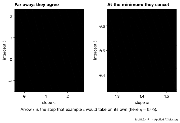
Each thin arrow is the step one example would take alone. Left: far from the minimum the four roughly agree, and the thick arrow is their average. Right: at the minimum they disagree and cancel exactly.
Far from the minimum, any single arrow points roughly the right way, and following it costs a quarter of the work. That is the bargain: a cheaper step that is a little wrong.
There are three ways to strike it. Batch gradient descent uses all \(n\) examples for every update. Stochastic gradient descent (SGD) uses one example, picked at random. A mini-batch method uses a small random handful, a set \(B\) of examples, and averages their gradients.
Build it up
Step 1. Split the gradient by example. Write \(L_i = (\hat{y}_i - y_i)^2\) for the squared error of example \(i\) alone. Then \(L\) is the average of the \(L_i\), and the gradient of \(L\) is the average of their gradients.
Step 2. Use one example. Pick an index \(i\) at random, each equally likely, and step against the gradient of \(L_i\) only. Sometimes the step is too long, sometimes too short, sometimes a little off course. On average it is exactly the full-batch step.
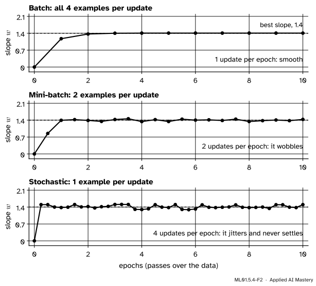
Step 3. Accept the noise. Because each step uses a different example, the path jitters. Near the minimum the jitter never dies away, since the single-example gradients are not zero there. With a fixed learning rate, SGD hovers round the minimum instead of settling on it.
ML01.5.4-F2
The slope \(w\) during ten epochs, from \((0, 0)\) with \(\eta = 0.05\). Fewer examples per update means more updates in the same time, and a path that never quite comes to rest.
Step 4. Average a few to calm it. A mini-batch of two examples gives a gradient that is the average of two opinions. It is noisier than the full gradient and steadier than a single example. The batch size is a dial between the two extremes.
Step 5. Organise the work into epochs. One epoch is one pass over the data. In practice you shuffle the examples, walk through the shuffled list one mini-batch at a time, and shuffle again before the next pass. Every example is then used exactly once per epoch. With \(n\) examples and batches of size \(\abs{B}\), an epoch contains \(n / \abs{B}\) updates (when \(\abs{B}\) divides \(n\)).
Method
Examples per update
Updates per epoch (\(n = 4\)), and path
Batch
\(n = 4\)
\(1\), smooth
Mini-batch
\(\abs{B} = 2\)
\(2\), wobbles
Stochastic
\(1\)
\(4\), jitters
The formal statement
NoteResult: the stochastic gradient is unbiased
Let \(L = \frac{1}{n} \sum_{i=1}^{n} L_i\), and let \(I\) be an index picked uniformly at random from \(1, \dots, n\). Then
In words: the gradient of one random example may be wrong every single time, but its average over all the ways the example could have been picked is the full gradient. An estimate with that property is called unbiased.
Step A: the gradient of one example. By the chain rule of lesson 2, applied to \(L_i = (w x_i + b - y_i)^2\) with no sum and no \(\frac{1}{n}\):
Check it at \((w, b) = (0, 0)\), where each residual is \(-y_i\). The four gradients are \((-4, -4)\), \((-12, -6)\), \((-30, -10)\) and \((-48, -12)\). Their average is \((-94/4,\ -32/4) = (-23.5, -8)\), the gradient computed by hand in lesson 2.
Step C: the expectation. An expectation is a sum over the possible outcomes, each weighted by its probability. Here the outcomes are \(I = 1, \dots, n\) and each has probability \(\frac{1}{n}\):
\[
\begin{aligned}
& \E[\nabla L_I] \\
&= \sum_{i=1}^{n} \Prob(I = i)\; \nabla L_i \\
&\quad\ \small\text{(definition of expectation)} \\
&= \sum_{i=1}^{n} \frac{1}{n}\, \nabla L_i \\
&\quad\ \small\text{(every index is equally likely)} \\
&= \frac{1}{n} \sum_{i=1}^{n} \nabla L_i \\
&\quad\ \small\text{(take out the constant)} \\
&= \nabla L \\
&\quad\ \small\text{(by Step B)}
\end{aligned}
\]
The second equality is where the uniform choice is used. Pick some examples more often than others and the result is no longer \(\nabla L\) (exercise 3).
Mini-batches are unbiased too. Let \(B\) be a set of \(m\) distinct indices, with every such set equally likely, and let \(\vect{g}_B = \frac{1}{m} \sum_{i \in B} \nabla L_i\). Write the sum over \(B\) as a sum over all examples with a switch \(s_i\) that is \(1\) if \(i\) is in \(B\) and \(0\) if not: \(\vect{g}_B = \frac{1}{m} \sum_{i=1}^{n} s_i\, \nabla L_i\). Every example is equally likely to be chosen, and \(m\) of the \(n\) are, so \(\E[s_i] = \Prob(i \in B) = \frac{m}{n}\). Therefore
What the batch size buys. Unbiased says nothing about how far a single draw can stray. At \((0, 0)\) the first component of the four gradients is \(-4, -12, -30, -48\): spread widely round \(-23.5\), with variance \(288.75\). For the six possible pairs it is \(-8, -17, -26, -21, -30, -39\): the same centre, with variance \(96.25\), a third as much. A larger batch gives a steadier gradient at a higher price per update.
Go deeper: how the noise shrinks with the batch size
If the single-example gradients have variance \(\sigma^2\) in some component, the average of \(m\) distinct examples drawn from \(n\) has variance
For \(n = 4\) and \(m = 2\) this is \(\frac{288.75}{2} \cdot \frac{2}{3} = 96.25\), as found above, and for \(m = n\) it is zero: the full batch has no noise at all. When \(n\) is far larger than \(m\) the second factor is close to \(1\), and the variance is close to \(\sigma^2 / m\). The typical size of the noise, its standard deviation, then falls like \(1 / \sqrt{m}\). A batch a hundred times larger costs a hundred times more per update and is only ten times steadier, one reason batches are kept small.
Why SGD does not settle. At the minimum \((1.4, 0.5)\) the residuals are \(-0.1,\ 0.3,\ -0.3,\ 0.1\), so by Step A the four gradients are \((-0.2, -0.2)\), \((1.2, 0.6)\), \((-1.8, -0.6)\) and \((0.8, 0.2)\). They add up to zero, which is what makes this point the minimum. None of them is zero itself. A stochastic step taken there moves away again. A smaller learning rate shrinks the hovering, and a learning rate that decays towards zero lets the run close in.
Go deeper: why a shuffled run hovers slightly to one side of the minimum
Unbiased describes one pick made independently of the path so far. In a shuffled epoch the picks depend on each other: after three examples, the fourth is certain. So the cloud is centred a little off the minimum: at \(\eta = 0.05\) the long-run average position at the end of an epoch is \((1.380, 0.528)\). The offset shrinks with \(\eta\).
Worked example
One epoch of stochastic gradient descent by hand, from \((0, 0)\) with \(\eta = 0.05\).
Suppose the shuffle gives the order: example 2, example 4, example 1, example 3. Each step uses Step A on one example, then the usual update.
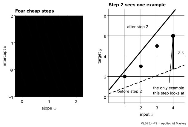
Left: the four steps, beside the single full-batch step that costs the same. Right: step 2 in data space. It looks at example 4 only, and swings the line up towards that one point without regard for the others.
The epoch cost four single-example gradients, the same as one full-batch step. The full-batch step from lesson 2 reached \((1.175, 0.4)\) with a loss of \(0.552\). The four cheap steps reached \((1.514, 0.458)\) with a loss of \(0.125\).
Code
First the formal section, checked exactly by listing every possible choice.
from itertools import combinationsimport numpy as npx = np.array([1.0, 2.0, 3.0, 4.0])y = np.array([2.0, 3.0, 5.0, 6.0])n =len(x)def loss(w, b):return np.mean((w * x + b - y) **2)def example_gradients(w, b):"""One row per example: the gradient of that example's squared error alone.""" residual = w * x + b - yreturn np.column_stack([2* residual * x, 2* residual])G = example_gradients(0.0, 0.0)pairs = np.array([G[[i, j]].mean(axis=0) for i, j in combinations(range(n), 2)])print("single examples:\n", G)print("their average: ", G.mean(axis=0))print("average over the 6 pairs:", pairs.mean(axis=0))print("variance of dL/dw: singles", G[:, 0].var(), " pairs", pairs[:, 0].var())print("at the minimum:\n", example_gradients(1.4, 0.5).round(10))
single examples:
 [[ -4.  -4.]
 [-12.  -6.]
 [-30. -10.]
 [-48. -12.]]
their average:   [-23.5  -8. ]
average over the 6 pairs: [-23.5  -8. ]
variance of dL/dw:  singles 288.75   pairs 96.25
at the minimum:
 [[-0.2 -0.2]
 [ 1.2  0.6]
 [-1.8 -0.6]
 [ 0.8  0.2]]
Now the algorithm. One function covers all three methods: batch_size=1 is stochastic, batch_size=n is full batch.
def run_epoch(w, b, lr, order, batch_size=1):"""One pass over the data in the given order, one update per mini-batch."""for k inrange(0, len(order), batch_size): batch = order[k:k + batch_size] dw, db = example_gradients(w, b)[batch].mean(axis=0) w, b = w - lr * dw, b - lr * dbreturn w, bdef minibatch_gd(w, b, lr, epochs, batch_size, seed=0): rng = np.random.default_rng(seed) # a fixed seed makes the run repeatablefor _ inrange(epochs): order = rng.permutation(n) # a fresh shuffle for every epoch w, b = run_epoch(w, b, lr, order, batch_size)return w, bhand_order = np.array([1, 3, 0, 2]) # examples 2, 4, 1, 3 (Python counts from 0)w_hand, b_hand = run_epoch(0.0, 0.0, 0.05, hand_order)print(f"the worked epoch: w = {w_hand:.3f}, b = {b_hand:.3f}, L = {loss(w_hand, b_hand):.3f}")for name, size in [("batch", 4), ("mini-batch", 2), ("stochastic", 1)]: w, b = minibatch_gd(0.0, 0.0, lr=0.02, epochs=200, batch_size=size)print(f"{name:<10} 200 epochs, {200* n // size:>3} updates: w = {w:.4f}, b = {b:.4f}, L = {loss(w, b):.5f}")
the worked epoch:  w = 1.514, b = 0.458, L = 0.125
batch       200 epochs, 200 updates:  w = 1.4022, b = 0.4936, L = 0.05001
mini-batch  200 epochs, 400 updates:  w = 1.3991, b = 0.5026, L = 0.05000
stochastic  200 epochs, 800 updates:  w = 1.3866, b = 0.5087, L = 0.05084
All three end near \((1.4, 0.5)\). The batch run is still creeping along the valley, and the stochastic run is hovering.
Finally the library. scikit-learn’s SGDRegressor is stochastic gradient descent for linear models. Set up to match, it reproduces the worked epoch.
from sklearn.linear_model import SGDRegressorX = x.reshape(-1, 1)same = SGDRegressor( loss="squared_error", penalty=None, learning_rate="constant", eta0=2*0.05, shuffle=False, max_iter=1, tol=None,)same.fit(X[hand_order], y[hand_order])print(f"SGDRegressor, one epoch in the same order: w = {same.coef_[0]:.3f}, b = {same.intercept_[0]:.3f}")usual = SGDRegressor(penalty=None, eta0=0.04, max_iter=2000, tol=None, random_state=0).fit(X, y)print(f"SGDRegressor, decaying rate, 2000 epochs: w = {usual.coef_[0]:.3f}, b = {usual.intercept_[0]:.3f}")
SGDRegressor, one epoch in the same order:  w = 1.514, b = 0.458
SGDRegressor, decaying rate, 2000 epochs:   w = 1.399, b = 0.500
Four things differ from the loop above.
The loss. scikit-learn’s squared error is \(\frac{1}{2}(\hat{y} - y)^2\), so its gradient has no factor \(2\). Its eta0 must be twice our \(\eta\) to take the same step, hence eta0=2 * 0.05.
The learning rate. By default it decays as eta0 / t**0.25, where t counts the updates. The second call uses this schedule and closes in on \((1.4, 0.5)\), where a constant rate hovers.
A penalty. By default a small penalty on the size of \(w\) is added (penalty="l2"). Both calls switch it off.
One example per update. There is no batch size to set. Shuffling is on by default and uses the library’s own random generator, so a shuffled run will not match ours step for step.
Explore
This module’s interactive, the gradient descent explorer, is in lesson 3. It runs full-batch gradient descent, so its paths are smooth.
Pitfalls
ML01.5.4-F4
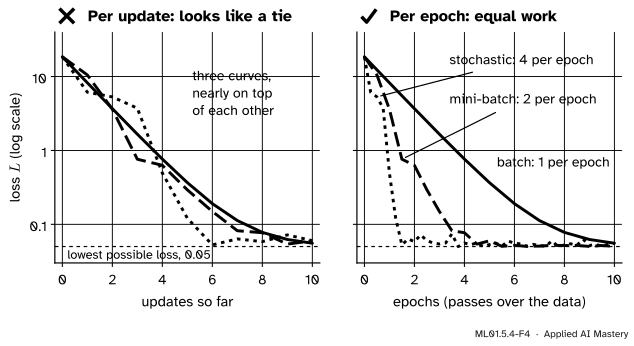
Wrong beside right, for the same three runs (\(\eta = 0.02\)). Counted in updates they look alike. Counted in epochs, which measure the work done, the cheap updates are far ahead.
“SGD took 400 updates and batch took 100, so batch is four times faster.”
An update is not a unit of work. A full-batch update here computes four single-example gradients and a stochastic update computes one. Compare runs by epochs, or by examples processed, and say which axis a loss curve uses.
“The data are already in a file, so I can go through them in order.”
The derivation needed a random pick. With a fixed order, the same sequence of pushes repeats every epoch and its errors do not average out. Run the four examples in the order 1, 2, 3, 4 with \(\eta = 0.05\) and the parameters at the end of each epoch settle at \((1.227, 0.829)\), with a loss of \(0.098\): a fixed spot that is not the minimum. Real files are often sorted by date, by class or by source, which is worse. Shuffle before every epoch.
ML01.5.4-F5
Where a stochastic run spends its time once it has arrived: 400 updates at a fixed learning rate. It hovers in a cloud, and a smaller learning rate gives a smaller cloud.
“The loss went up on that step, so something is broken.”
On this bowl, with full-batch steps below the limit of lesson 3, the loss never rises. With stochastic steps it rises all the time, and that is expected. Stand exactly at the minimum, take one step on example 3 with \(\eta = 0.05\), and the loss goes from \(0.05\) to \(0.125\). Judge a stochastic run by its trend over epochs. To reduce the noise, lower the learning rate, enlarge the batch, or let the rate decay.
Check yourself
Recall
1. How is the full gradient related to the gradients of the single examples?
Show answer
It is their average: \(\nabla L = \frac{1}{n} \sum_i \nabla L_i\).
2. What does it mean that the stochastic gradient is unbiased, and what assumption makes it so?
Show answer
Its expectation is the full gradient, \(\E[\nabla L_I] = \nabla L\). This needs the index \(I\) to be picked uniformly at random, each example with probability \(\frac{1}{n}\).
3. How many examples does one update use in batch, stochastic and mini-batch gradient descent?
Show answer
All \(n\); one; and a small set \(B\) of \(\abs{B}\) examples.
4. What is an epoch, and how many updates does it contain?
Show answer
One pass over the data, in which every example is used once. It contains \(n / \abs{B}\) updates.
5. Why does SGD with a fixed learning rate hover round the minimum instead of settling on it?
Show answer
At the minimum the single-example gradients cancel on average but are not zero one by one, so every step still moves the parameters.
Exercises
1.★ At \((w, b) = (1, 0)\), compute the gradient of each example and check that their average is the full gradient \((-8.5, -3)\).
Show solution
The predictions are \(1, 2, 3, 4\) and the residuals \(-1, -1, -2, -2\). Using \(\nabla L_i = (2 r_i x_i,\ 2 r_i)\): \((-2, -2)\), \((-4, -2)\), \((-12, -4)\) and \((-16, -4)\). The average is \((-34/4,\ -12/4) = (-8.5, -3)\).
2.★★ From \((0, 0)\) with \(\eta = 0.05\), take one mini-batch step with \(B = \{1, 4\}\), and separately one with \(B = \{2, 3\}\). Where does each land? Average the two landing points and explain what you find.
Show solution
For \(B = \{1, 4\}\) the mini-batch gradient is the average of \((-4, -4)\) and \((-48, -12)\), which is \((-26, -8)\). The step lands at \((0.05 \cdot 26,\ 0.05 \cdot 8) = (1.3, 0.4)\).
For \(B = \{2, 3\}\) it is the average of \((-12, -6)\) and \((-30, -10)\), which is \((-21, -8)\). The step lands at \((1.05, 0.4)\).
The average of the landing points is \((1.175, 0.4)\), exactly the full-batch step of lesson 2. The two batches together contain every example once, so the average of their two gradients is the average over all four examples, the full gradient.
3.★★★ Suppose the sampling is not uniform: example 4 is picked with probability \(\frac{1}{2}\) and each of the others with probability \(\frac{1}{6}\). Compute \(\E[\nabla L_I]\) at \((0, 0)\) and compare it with the full gradient. Then show that weighting the gradient of example \(i\) by \(\frac{1}{n\,p_i}\), where \(p_i\) is its probability, removes the bias for any choice of positive probabilities.
Show solution
\(\E[\nabla L_I] = \frac{1}{6}\big[ (-4, -4) + (-12, -6) + (-30, -10) \big] + \frac{1}{2}(-48, -12)
= (-7.67, -3.33) + (-24, -6) = (-31.67, -9.33)\). The full gradient is \((-23.5, -8)\), so this estimate is biased: example 4 is heard too often.
The probability \(p_i\) cancels. Examples that are picked more often count for less each time. Uniform sampling is the case \(p_i = \frac{1}{n}\), where every weight is \(1\).
Summary card
One example gives a cheap, noisy step that is right on average.
ML01.5.4-F1
Four opinions, one average.
Average.\(\nabla L = \frac{1}{n} \sum_i \nabla L_i\) with \(\nabla L_i = \big( 2(\hat{y}_i - y_i)\,x_i,\ 2(\hat{y}_i - y_i) \big)\).
Unbiased. For \(I\) uniform on \(1, \dots, n\): \(\E[\nabla L_I] = \nabla L\). The same holds for a uniformly chosen mini-batch.
The dial. Batch: \(n\) per update, smooth. Stochastic: \(1\) per update, jitters. Mini-batch: \(\abs{B}\) per update, in between.
Epoch. One shuffled pass over the data: \(n / \abs{B}\) updates.
Fixed rate. SGD hovers round the minimum. A smaller or decaying rate, or a larger batch, tightens the cloud.
Sources and next steps
Sources. Each was opened and checked against this lesson on 12 November 2026.
Aston Zhang, Zachary Lipton, Mu Li and Alexander Smola, Dive into Deep Learning, Section 12.4. Equations (12.4.1) to (12.4.4) give the objective as an average over examples, the stochastic update, and the unbiasedness of the stochastic gradient. Section 12.4.4 notes that practice samples without replacement. Section 12.5.2 states that the standard deviation of the mini-batch gradient falls by a factor of \(b^{-1/2}\) for batch size \(b\).
Ian Goodfellow, Yoshua Bengio and Aaron Courville, Deep Learning, MIT Press, 2016, Section 8.1.3. Gives the names batch, stochastic and minibatch, the less-than-linear return of larger batches, and the need to pick minibatches randomly and to shuffle ordered data.
Tengyu Ma and Andrew Ng, CS229 Lecture Notes, Stanford University, Section 1.1. Contrasts batch gradient descent (1.1) with stochastic gradient descent (1.2), whose parameters keep oscillating around the minimum unless the learning rate is slowly decreased.
Google, Machine Learning Crash Course, Linear regression: Hyperparameters. Defines batch size, stochastic and mini-batch gradient descent, noise and the epoch.
scikit-learn 1.9 documentation, SGDRegressor and the user guide, Section 1.5. The class page lists the defaults quoted above. Section 1.5.8 gives the squared error with its factor \(\frac{1}{2}\).
Next. Module ML01.6, logistic regression and classification, keeps this training loop and changes only the model and the loss.