On a quadratic loss, every gradient descent step multiplies the distance to the minimum by one fixed number. From that, find exactly which learning rates crawl, converge, oscillate or diverge, tie the limit to the data, and see why standardising the input helps.
Derive that one gradient descent step on a one-parameter quadratic multiplies the distance to the minimum by 1 minus the learning rate times the curvature.
State which learning rates crawl, converge, oscillate and diverge, with the exact limit of 2 over the curvature.
Compute the curvature of a loss from the data, and the limit for two parameters from the matrix of second derivatives.
Explain why standardising the input makes the bowl round and allows a larger learning rate.
In review. The maths and code on this page are checked by automated tests on every change, but an independent reader has not signed it off yet. Spot a mistake or a confusing step? Tell us.
The question
In the last lesson a learning rate of \(0.05\) took the loss from \(18.5\) to \(0.55\) in one step. So would \(0.5\) be ten times faster? Try it, and after ten steps the loss is about \(4 \times 10^{18}\). Somewhere between \(0.05\) and \(0.5\) gradient descent stops working. Where exactly is the line, what decides it, and can it be moved? The learning rate is the first setting anyone tunes when a model will not train.
From the last lesson
1. State the update rule and name \(\eta\).
Show answer
\(w \leftarrow w - \eta\, \pd{L}{w}\) and \(b \leftarrow b - \eta\, \pd{L}{b}\), both computed at the current point. \(\eta\) is the learning rate.
2. Which way does the gradient point on the loss map?
Show answer
Straight uphill, at a right angle to the contour lines. The update steps the opposite way.
Intuition
The update moves each parameter by \(\eta\) times a slope. The slope says which way to go and how steep the ground is. The learning rate\(\eta\) turns that into a distance. The slope comes from the data. The learning rate is your choice.
ML01.5.3-F1
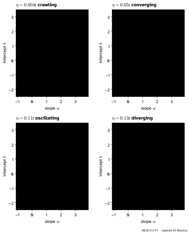
One bowl, one starting point, four learning rates, 40 steps each. Too small and the run crawls. A moderate rate converges. A larger one oscillates across the valley but still closes in. Past a sharp limit the run diverges.
The four pictures differ in one number only. This lesson finds the exact boundaries between them, starting in one dimension.
Build it up
Step 1. Strip the problem down to one parameter. Freeze the intercept at \(b = 0.5\). Exercise 2 of lesson 1 found this slice of the bowl:
\[
L(w) = 7.5\,(w - 1.4)^2 + 0.05 .
\]
It is a parabola with its bottom at \(w = 1.4\). Its slope is \(\frac{dL}{dw} = 15\,(w - 1.4)\).
Step 2. Write one update in terms of the distance to the bottom. The update is \(w_{\text{new}} = w - \eta \cdot 15\,(w - 1.4)\). Subtract \(1.4\) from both sides:
The distance to the bottom is multiplied by \(1 - 15\eta\), the same multiplier at every step.
Step 3. Read the behaviour off the multiplier. If the multiplier is \(0.4\), each step leaves \(40\%\) of the distance and the run closes in from one side. If it is \(-0.5\), the distance halves but changes sign: the run jumps over the bottom and lands closer on the far side. If it is \(-1.1\), every jump lands further away than the last.
ML01.5.3-F2
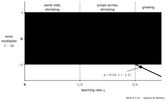
The multiplier \(1 - \eta h\) for every learning rate, drawn for a parabola of curvature \(h\) (here \(h = 15\)). The run converges exactly while the green line is inside the shaded band.
Step 4. With two parameters, the steepest direction sets the limit. A bowl curves by different amounts in different directions. Ours is steep across the valley and nearly flat along it. One learning rate has to serve both, so it must be small enough for the steep direction. The flat direction then gets steps that are far smaller than it could take. That is the creep along the valley floor in the figure above.
Step 5. Make the bowl round. If every direction curved equally, one learning rate would suit them all. Rescaling the input does exactly that.
The formal statement
NoteResult: gradient descent on a one-parameter quadratic
Let \(L(w) = \frac{h}{2}(w - w^*)^2 + c\) with curvature\(h > 0\), and run \(w_{t+1} = w_t - \eta\, \frac{dL}{dw}(w_t)\). Then
Apply this \(t\) times from \(w_0\) and the factor \((1 - \eta h)\) appears \(t\) times: the second formula. A power \(m^t\) shrinks to zero exactly when \(-1 < m < 1\). With \(m = 1 - \eta h\):
The regimes. Reading the multiplier \(m = 1 - \eta h\) from left to right in the figure:
Learning rate
Multiplier \(m\)
What the run does
\(\eta\) close to \(0\)
just below \(1\)
Crawls: each step removes a sliver of the distance
\(0 < \eta < 1/h\)
\(0 < m < 1\)
Converges from one side
\(\eta = 1/h\)
\(0\)
Lands on the bottom in one step
\(1/h < \eta < 2/h\)
\(-1 < m < 0\)
Oscillates: jumps across the bottom, closer each time
\(\eta = 2/h\)
\(-1\)
Bounces between two points for ever
\(\eta > 2/h\)
\(m < -1\)
Diverges: each jump is longer than the last
Crawling is a matter of degree. The other boundaries are sharp.
The loss in the oscillating regime. The loss above its minimum is \(L(w_t) - c = \frac{h}{2}(w_t - w^*)^2\), so each step multiplies it by \(m^2\). While \(-1 < m < 1\) that is less than \(1\). The parameter may jump from side to side, but the loss falls at every single step.
Where \(h\) comes from. Lesson 1 showed that with \(b\) fixed, \(L(w) = A w^2 - B w + C\) with \(A = \frac{1}{n} \sum_i x_i^2\). Matching the coefficient of \(w^2\) with \(\frac{h}{2}\) gives
The curvature depends only on the inputs. For the running example \(h = \frac{2}{4} \cdot 30 = 15\), so the run lands in one step at \(\eta = 1/15 \approx 0.067\) and the limit is \(\eta = 2/15 \approx 0.133\).
Two parameters. Differentiate the two slopes of lesson 2 once more. The slope \(\pd{L}{w} = \frac{2}{n} \sum_i (w x_i + b - y_i)\, x_i\) changes at the rate \(\frac{2}{n} \sum_i x_i^2\) as \(w\) moves and \(\frac{2}{n} \sum_i x_i\) as \(b\) moves. The slope \(\pd{L}{b} = \frac{2}{n} \sum_i (w x_i + b - y_i)\) changes at the rate \(\frac{2}{n} \sum_i x_i\) as \(w\) moves and \(\frac{2}{n} \cdot n = 2\) as \(b\) moves. These four second derivatives form the Hessian:
The bowl has a steepest direction, across the valley, and a flattest direction, along it. Cut the bowl along either and you get a parabola. Their curvatures are the two eigenvalues of \(\mat{H}\), the solutions of \((15 - \lambda)(2 - \lambda) - 5 \cdot 5 = 0\), that is \(\lambda^2 - 17\lambda + 5 = 0\):
Along each of these two directions the one-parameter result holds, with \(h\) replaced by that direction’s eigenvalue. The run converges only if it converges in both, and the steeper one is the stricter:
The flat direction pays for it. Even at the limit its multiplier is \(1 - 0.1198 \cdot 0.30 \approx 0.964\), so no allowed learning rate removes more than about \(3.6\%\) of the distance along the valley per step. The ratio \(\lambda_{\max} / \lambda_{\min} \approx 56\) is the condition number of the bowl. The larger it is, the longer and narrower the valley and the slower gradient descent.
Go deeper: why each direction of the bowl behaves like its own parabola
For a quadratic loss with minimum \(\vect{p}^* = (w^*, b^*)\), the gradient at \(\vect{p} = (w, b)\) is \(\nabla L = \mat{H}(\vect{p} - \vect{p}^*)\). Check it at \((0, 0)\): \(\mat{H}\,(-1.4, -0.5) = (15 \cdot (-1.4) + 5 \cdot (-0.5),\; 5 \cdot (-1.4) + 2 \cdot (-0.5)) = (-23.5, -8)\), the gradient found by hand in lesson 2. The update therefore reads
An eigenvector of \(\mat{H}\) is a direction \(\vect{v}\) that \(\mat{H}\) only stretches: \(\mat{H}\vect{v} = \lambda \vect{v}\). For \(\vect{v} = (v_1, v_2)\) that reads \((15 - \lambda)\,v_1 + 5\,v_2 = 0\) and \(5\,v_1 + (2 - \lambda)\,v_2 = 0\). Multiply the first by \((2 - \lambda)\) and the second by \(5\), then subtract:
If \(v_1\) were zero, the first equation would make \(v_2\) zero too. So the bracket is zero: the equation solved above.
A symmetric matrix such as \(\mat{H}\) has two eigenvectors, at right angles, so any distance from the minimum can be written as \(\vect{p}_t - \vect{p}^* = a_t \vect{v}_1 + c_t \vect{v}_2\). Substituting,
The two parts never mix. Each is multiplied by its own \(1 - \eta \lambda\), exactly as in one dimension. Here \(\vect{v}_{\max} \approx (0.95, 0.32)\) points across the valley and \(\vect{v}_{\min} \approx (-0.32, 0.95)\) along it.
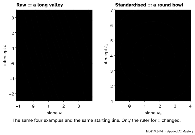
Standardising the input. Replace each \(x_i\) by \(z_i = (x_i - \bar{x}) / s\), where \(\bar{x}\) is the mean of the inputs and \(s\) their standard deviation. Here \(\bar{x} = 2.5\) and \(s = \sqrt{1.25} \approx 1.118\), so \(z = (-1.342,\ -0.447,\ 0.447,\ 1.342)\). By construction \(\sum_i z_i = 0\) and \(\frac{1}{n} \sum_i z_i^2 = 1\). Fit \(\hat{y} = w_z z + b_z\) instead, and the Hessian becomes
Both curvatures are \(2\). The contour lines are circles, the condition number is \(1\), the limit rises from \(0.1198\) to \(2/2 = 1\), and \(\eta = 1/2\) lands on the minimum in one step from anywhere. It is the same line as before, written for the new ruler: \(w_z = 1.4\,s \approx 1.565\) and \(b_z = 0.5 + 1.4\,\bar{x} = 4\).
ML01.5.3-F4
Left: on the raw input the best the run can do is zigzag and creep. Right: on the standardised input every contour is a circle, the downhill direction points at the minimum, and a learning rate four times larger goes straight there.
Worked example
Three learning rates on the parabola \(L(w) = 7.5\,(w - 1.4)^2 + 0.05\), each from \(w_0 = 0\).
Here \(h = 15\), so the boundaries are \(1/h \approx 0.067\) and \(2/h \approx 0.133\).
The first step for \(\eta = 0.1\), the long way. The slope at \(w_0 = 0\) is \(15 \cdot (0 - 1.4) = -21\). The update gives \(w_1 = 0 - 0.1 \cdot (-21) = 2.1\). The run has jumped over the bottom at \(1.4\).
The same step with the multiplier.\(1 - \eta h = 1 - 0.1 \cdot 15 = -0.5\). The starting distance is \(0 - 1.4 = -1.4\), the new one is \(-0.5 \cdot (-1.4) = 0.7\), and \(1.4 + 0.7 = 2.1\).
The multiplier does the rest, one column per rate:
\(\eta\)
\(0.04\)
\(0.1\)
\(0.14\)
\(1 - \eta h\)
\(0.4\)
\(-0.5\)
\(-1.1\)
\(w_0\)
\(0\)
\(0\)
\(0\)
\(w_1\)
\(0.84\)
\(2.1\)
\(2.94\)
\(w_2\)
\(1.176\)
\(1.05\)
\(-0.294\)
\(w_3\)
\(1.3104\)
\(1.575\)
\(3.2634\)
\(L(w_0)\)
\(14.75\)
\(14.75\)
\(14.75\)
\(L(w_1)\)
\(2.402\)
\(3.725\)
\(17.837\)
\(L(w_2)\)
\(0.426\)
\(0.969\)
\(21.572\)
\(L(w_3)\)
\(0.110\)
\(0.280\)
\(26.092\)
ML01.5.3-F3
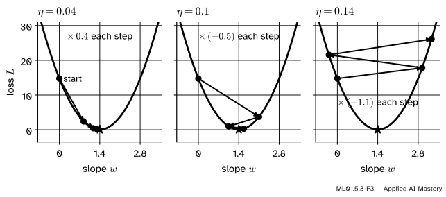
The table as a picture. With \(\eta = 0.04\) the run approaches from one side. With \(\eta = 0.1\) it jumps across and still descends. With \(\eta = 0.14\), just past the limit of \(0.133\), it climbs.
In the middle column \(w\) swings from \(2.1\) to \(1.05\) to \(1.575\), yet the loss falls every time, by the factor \((-0.5)^2 = 0.25\) above its floor of \(0.05\). In the last column the loss grows by \((-1.1)^2 = 1.21\) above that floor at each step.
Code
The one-parameter run from scratch, checked against the table and the closed form.
import numpy as nph, w_star, c =15.0, 1.4, 0.05# the slice b = 0.5def loss_1d(w):return0.5* h * (w - w_star) **2+ cdef descend_1d(w, lr, steps): path = [w]for _ inrange(steps): w = w - lr * h * (w - w_star) # slope = h * (w - w_star) path.append(w)return np.array(path)for lr in [0.04, 0.1, 0.14]: path = descend_1d(0.0, lr, 3)print(f"lr = {lr:<5} multiplier = {1- lr * h:+.1f} w: {np.round(path, 4)} "f"L: {np.round(loss_1d(path), 3)}")
Now two parameters: the Hessian from the data, its eigenvalues by the quadratic formula and by NumPy, and the limit tested from both sides.
x = np.array([1.0, 2.0, 3.0, 4.0])y = np.array([2.0, 3.0, 5.0, 6.0])def loss(w, b, x=x):return np.mean((w * x + b - y) **2)def descend(w, b, lr, steps, x=x):for _ inrange(steps): residual = w * x + b - y w, b = w - lr *2* np.mean(residual * x), b - lr *2* np.mean(residual)return w, bdef hessian(x):return np.array([[2* np.mean(x **2), 2* np.mean(x)], [2* np.mean(x), 2.0]])H = hessian(x)by_hand = (17- np.sqrt(269)) /2, (17+ np.sqrt(269)) /2lam_min, lam_max = np.linalg.eigvalsh(H)limit =2/ lam_maxprint("Hessian:\n", H)print(f"eigenvalues: {lam_min:.4f} and {lam_max:.4f} condition number: {lam_max / lam_min:.1f}")print(f"limit 2 / lam_max = {limit:.4f}")for lr in [0.99* limit, 1.01* limit]: w, b = descend(0.0, 0.0, lr, 2000)print(f"lr = {lr:.4f}: loss after 2000 steps = {loss(w, b):.3g}")print(f"lr = 0.5: loss after 10 steps = {loss(*descend(0.0, 0.0, 0.5, 10)):.3g}")
Hessian:
 [[15.  5.]
 [ 5.  2.]]
eigenvalues: 0.2994 and 16.7006   condition number: 55.8
limit 2 / lam_max = 0.1198
lr = 0.1186: loss after 2000 steps = 0.05
lr = 0.1210: loss after 2000 steps = 4.64e+35
lr = 0.5:    loss after 10 steps   = 3.91e+18
Finally, standardise. First by hand, then with scikit-learn’s StandardScaler, which does the same subtraction and division.
from sklearn.preprocessing import StandardScalermean, sd = x.mean(), x.std() # 2.5 and sqrt(1.25)z = (x - mean) / sdcolumn = x.reshape(-1, 1) # one row per example, one column per featurescaler = StandardScaler().fit(column)z_library = scaler.transform(column)[:, 0]print("z =", np.round(z, 3))print("Hessian for z:\n", hessian(z).round(12) +0.0) # + 0.0 turns -0.0 into 0.0w_z, b_z = descend(0.0, 0.0, 0.5, 1, x=z) # one step at lr = 1/2print(f"one step at lr = 0.5: w_z = {w_z:.4f}, b_z = {b_z:.4f}, loss = {loss(w_z, b_z, x=z):.4f}")print(f"back on the raw ruler: w = {w_z / sd:.4f}, b = {b_z - w_z * mean / sd:.4f}")def steps_needed(w, b, lr, x):"""Steps until the loss is within one millionth of its lowest value, 0.05.""" steps =0while loss(w, b, x) -0.05>1e-6: (w, b), steps = descend(w, b, lr, 1, x), steps +1return stepsstart = (-0.3, 2.0) # the starting line of the figuresstart_z = (start[0] * sd, start[1] + start[0] * mean) # the same line, written for zprint("raw x, lr = 0.1:", steps_needed(*start, 0.1, x), "steps")print("standardised x, lr = 0.4:", steps_needed(*start_z, 0.4, z), "steps")
z = [-1.342 -0.447  0.447  1.342]
Hessian for z:
 [[2. 0.]
 [0. 2.]]
one step at lr = 0.5: w_z = 1.5652, b_z = 4.0000, loss = 0.0500
back on the raw ruler: w = 1.4000, b = 0.5000
raw x,          lr = 0.1: 219 steps
standardised x, lr = 0.4: 6 steps
The same starting line needs 219 steps on the raw input and 6 on the standardised one. Only the shape of the bowl changed.
Explore
ML01.5-X1
Gradient descent explorer
Press Step a few times, then Run, and watch the read-out name the regime. Raise the learning rate until the path zigzags and then, just past the limit, flies off the map. Tap the map to start somewhere else, then switch on Standardise x and try the rates that failed before.
The run changes character exactly at the limit in the read-out, \(2/\lambda_{\max}\). From a start near the top of the map, every rate below it ends in a creep along the valley floor. With the input standardised, \(\eta = 0.5\) lands in one step. The loss chart is logarithmic: each gridline is ten or more times the one below.
Pitfalls
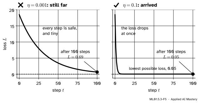
ML01.5.3-F5
Wrong beside right, for a budget of 100 steps from \((0, 0)\). The tiny rate never misbehaves and never arrives. The larger one arrives within a few steps.
“A smaller learning rate is always safer.”
It is safe from divergence, and that is all. With \(\eta = 0.001\) the loss after 100 steps is \(0.69\), fourteen times the lowest possible value, and nothing in the smooth curve warns you. Training budgets are finite, so too small fails as surely as too large. It just fails quietly.
“The loss went up, so the code is broken.”
Check the learning rate first. On this bowl, with the full gradient, the loss falls at every step for every rate below \(2/\lambda_{\max}\). Above it the loss sooner or later rises at every step, unless the start is exactly on the valley floor. A rising loss with a gradient that passes the finite-difference check means the rate is too large. Halve it and look again.
“\(\eta = 0.05\) worked here, so it will work on my data.”
The limit is \(2/\lambda_{\max}\), and the curvature comes from the inputs. Measure \(x\) in units ten times smaller and every \(x_i\) is ten times larger, \(h\) is a hundred times larger, and the limit falls from \(0.1198\) to \(0.0013\), about ninety times smaller. This is the practical reason to standardise inputs.
Check yourself
Recall
1. On a parabola with curvature \(h\), what does one gradient descent step do to the distance from the minimum?
Show answer
It multiplies it by \(1 - \eta h\): \(w_{t+1} - w^* = (1 - \eta h)(w_t - w^*)\).
2. For which learning rates does the run converge?
Show answer
Exactly for \(0 < \eta < 2/h\), because that is when \(-1 < 1 - \eta h < 1\).
3. What happens at \(\eta = 1/h\), and between \(1/h\) and \(2/h\)?
Show answer
At \(1/h\) the multiplier is zero and the run lands on the minimum in one step. Between \(1/h\) and \(2/h\) the multiplier is negative: the run jumps across the minimum each step but gets closer, and the loss still falls.
4. With two parameters, which curvature sets the limit, and what is the limit for the running example?
Show answer
The largest one, \(\lambda_{\max}\), the curvature of the steepest direction. The limit is \(2/\lambda_{\max} = 2/16.70 \approx 0.1198\).
5. What does standardising the input do to the bowl and to the limit?
Show answer
It makes the Hessian \(2\) on the diagonal and \(0\) elsewhere, so the contours become circles. The limit becomes \(1\), and \(\eta = 1/2\) reaches the minimum in one step.
Exercises
1.★ On the parabola \(L(w) = 7.5\,(w - 1.4)^2 + 0.05\), take \(\eta = 0.02\) and \(w_0 = 0\). Find the multiplier, \(w_1\) and \(w_2\). How many steps until the distance to the bottom is below \(1\%\) of where it started?
Show solution
The multiplier is \(1 - 0.02 \cdot 15 = 0.7\). The distances are \(-1.4\), then \(0.7 \cdot (-1.4) = -0.98\), then \(0.7 \cdot (-0.98) = -0.686\), so \(w_1 = 0.42\) and \(w_2 = 0.714\). After \(t\) steps the distance is \(0.7^t\) of its start. We need \(0.7^t < 0.01\), that is \(t > \ln 0.01 / \ln 0.7 \approx 12.9\), so \(13\) steps.
2.★★ The same four inputs are recorded in a unit ten times smaller, so \(x = 10, 20, 30, 40\), and the intercept is held fixed. Find the curvature \(h\) of the loss in \(w\) and the largest learning rate that converges. What does \(\eta = 0.05\) do now?
Show solution
\(h = \frac{2}{n} \sum_i x_i^2 = \frac{2}{4}(100 + 400 + 900 + 1600) = 1500\), a hundred times the old value of \(15\). The limit is \(2/1500 \approx 0.00133\). With \(\eta = 0.05\) the multiplier is \(1 - 0.05 \cdot 1500 = -74\): each step lands \(74\) times further from the bottom, on the other side. The rate that worked before now diverges violently.
3.★★★ Show that for any dataset whose inputs are not all equal, fitting \(\hat{y} = w_z z + b_z\) to the standardised input gives the Hessian \(\begin{bmatrix} 2 & 0 \\ 0 & 2 \end{bmatrix}\), and that gradient descent with \(\eta = 1/2\) then reaches the minimum in one step from any start. You may use that the gradient of a quadratic loss is \(\mat{H}(\vect{p} - \vect{p}^*)\).
Show solution
Let \(\bar{x} = \frac{1}{n} \sum_i x_i\) and \(s^2 = \frac{1}{n} \sum_i (x_i - \bar{x})^2\), which is positive because the inputs are not all equal. With \(z_i = (x_i - \bar{x})/s\),
The Hessian has entries \(\frac{2}{n} \sum_i z_i^2 = 2\), \(\frac{2}{n} \sum_i z_i = 0\) (twice) and \(2\). So \(\mat{H}\vect{v} = 2\vect{v}\) for every vector \(\vect{v}\), and the gradient is \(2(\vect{p} - \vect{p}^*)\). One update with \(\eta = 1/2\) gives
The result does not depend on the targets or on the starting point.
Summary card
Each step multiplies the distance to the minimum by \(1 - \eta h\).
ML01.5.3-F1
Crawl, converge, oscillate, diverge.
One parameter.\(w_t - w^* = (1 - \eta h)^t (w_0 - w^*)\). Converges exactly when \(0 < \eta < 2/h\).
Regimes. One step at \(\eta = 1/h\). Oscillates, and still converges, for \(1/h < \eta < 2/h\). Diverges beyond.
Curvature from data.\(h = \frac{2}{n} \sum_i x_i^2\), which is \(15\) here.
Two parameters. The limit is \(2/\lambda_{\max}\) of the Hessian \(\begin{bmatrix} 15 & 5 \\ 5 & 2 \end{bmatrix}\): \(2/16.70 \approx 0.1198\). The flat direction, \(\lambda_{\min} \approx 0.30\), sets the speed.
Standardise.\(z_i = (x_i - \bar{x})/s\) makes the Hessian \(2\) on the diagonal: a round bowl, limit \(1\), one step at \(\eta = 1/2\).
Sources and next steps
Sources. Each was opened and checked against this lesson on 12 November 2026.
Gabriel Goh, Why Momentum Really Works, Distill, 2017, section “First Steps: Gradient Descent”. Solves gradient descent on a convex quadratic in closed form: along each eigenvector the error is multiplied by \(1 - \alpha \lambda_i\) per step, the workable step sizes satisfy \(0 < \alpha \lambda_i < 2\), and the condition number is the ratio of the largest to the smallest eigenvalue.
Yann LeCun, Léon Bottou, Genevieve Orr and Klaus-Robert Müller, Efficient BackProp, 1998. Section 5.1 gives \(\eta < 2/\lambda_{\max}\) (equation 38) and \(\eta_{\text{opt}} = 1/\lambda_{\max}\) (39). Section 4.3 recommends inputs with a mean close to zero and about the same variance.
Ian Goodfellow, Yoshua Bengio and Aaron Courville, Deep Learning, MIT Press, 2016, Section 4.3.1. States that gradient descent performs poorly when the Hessian has a poor condition number.
Aston Zhang, Zachary Lipton, Mu Li and Alexander Smola, Dive into Deep Learning, Section 12.3.1.1. Shows on \(f(x) = x^2\) that too small a learning rate is slow and too large a one diverges.
Google, Machine Learning Crash Course, Linear regression: Hyperparameters. Describes a learning rate that is too low as slow to converge and one that is too high as never converging.
scikit-learn 1.9 documentation, StandardScaler. Computes \(z = (x - u)/s\) from the mean \(u\) and the standard deviation \(s\) (with ddof=0).