Set both partial derivatives of the mean squared error to zero and solve, one step at a time. The best slope is the covariance of x and y divided by the variance of x, and the best line passes through the point of means. Worked by hand on the course’s four points.
Differentiate the mean squared error of a line with respect to the intercept and the slope, holding the other fixed.
Solve the two resulting equations to get the slope as covariance over variance and the intercept through the means.
Compute the least-squares line of a small dataset by hand from a table of deviations.
State what the two equations say about the residuals: they sum to zero, and so do the residuals times x.
Say when the formula has no answer and why its answer is a minimum.
In review. The maths and code on this page are checked by automated tests on every change, but an independent reader has not signed it off yet. Spot a mistake or a confusing step? Tell us.
The question
You could hunt for the best line by trying thousands of candidates and keeping the one with the lowest loss. For a line scored by squared error you do not have to. Two equations, solved once, give the best slope and intercept exactly. Where do those equations come from, and why is the answer built from two statistics, a covariance and a variance? This is one of the few models whose training has an exact formula, so it is the yardstick that every other training method is checked against.
From the last lesson
1. What is the residual of an example, and how does the mean squared error use it?
Show answer
The residual is the prediction minus the target, \(r_i = \hat{y}_i - y_i\). The mean squared error is the mean of the squared residuals, \(L = \frac{1}{n} \sum_i r_i^2\).
2. If the same number must be predicted for every example, which number has the lowest mean squared error?
Show answer
The mean of the targets, \(\bar{y}\).
Intuition
The four points never change. What changes is the pair \((w, b)\), and each pair has a loss. So the mean squared error is a function of two numbers, \(L(w, b)\).
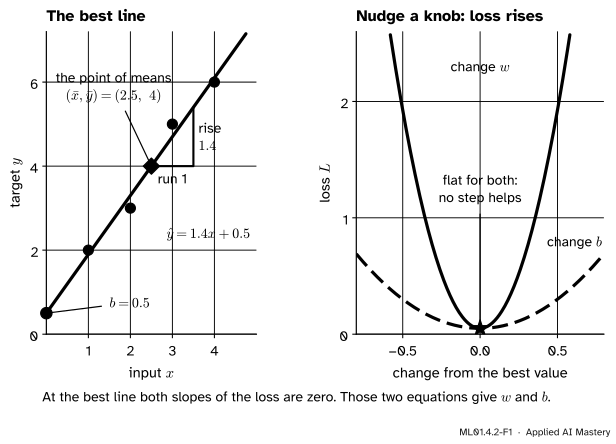
Stand at the best pair and nudge one parameter. If the loss could fall, the pair would not be the best. So at the best pair a small change of \(b\) alone does not lower the loss, and neither does a small change of \(w\) alone: the loss is flat in both directions. “Flat” means a slope of zero. Two parameters, two slopes, two equations.
ML01.4.2-F1
Left: the answer this lesson derives. The best line passes through the point of means and has slope \(1.4\). Right: why it is the best. Move \(w\) away from \(1.4\), or \(b\) away from \(0.5\), and the loss can only rise. At the bottom both curves are flat.
Solving the two equations gives two plain facts. The best line passes through the point of means\((\bar{x}, \bar{y})\). And its slope is how much \(x\) and \(y\) vary together, divided by how much \(x\) varies on its own.
Build it up
Step 1. Two slopes of one loss. The loss depends on two parameters, so it has two slopes. Hold \(w\) still and ask how fast \(L\) changes as \(b\) moves: that is the partial derivative\(\pd{L}{b}\). Hold \(b\) still and move \(w\): that is \(\pd{L}{w}\). Each is an ordinary derivative in which the other parameter is treated as a constant. Module M04.10, Partial derivatives, a first look, draws this idea as slices of a surface.
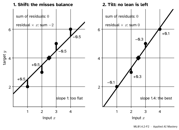
Step 2. The first equation: slide the line. Fix the slope at \(w = 1\) and slide the line up and down. If the line is mostly above the points, the residuals are mostly positive, and moving it down helps. If it is mostly below, moving it up helps. It stops helping when the positive and negative residuals balance: when they sum to zero. For \(w = 1\) that happens at \(b = 1.5\), which is line Q of the last lesson, with residuals \(0.5, 0.5, -0.5, -0.5\).
Step 3. The second equation: tilt the line. Line Q is balanced but still leans the wrong way. It is too high on the left, where \(x\) is small, and too low on the right, where \(x\) is large. Weight each residual by its \(x\) and the lean shows up as a number:
A negative total means the line is too low where \(x\) is large, so it should be steeper. Tilt it until this total is zero as well. That happens at slope \(1.4\).
ML01.4.2-F2
The two equations as two balances. Left: sliding has made the residuals sum to zero, but they still lean. Right: tilting about the point of means removes the lean. Now no slide and no tilt can lower the loss.
The formal section turns “balance” and “lean” into the two partial derivatives, and solves.
\[
L(w, b) = \frac{1}{n} \sum_{i=1}^{n} (w x_i + b - y_i)^2 .
\]
The slope with respect to \(b\). Take one term of the sum. By the chain rule, the derivative of a square is twice the inside, times the derivative of the inside. The inside is \(w x_i + b - y_i\), and its derivative with respect to \(b\) is \(1\):
\[
\begin{aligned}
&\pd{}{b} (w x_i + b - y_i)^2 \\
&\quad = 2\,(w x_i + b - y_i) \cdot 1 .
\end{aligned}
\]
Average over the examples, then take the mean of each of the three terms inside the bracket:
\[
\begin{aligned}
\pd{L}{b} &= \frac{2}{n} \sum_i (w x_i + b - y_i) \\
&= 2\,(w \bar{x} + b - \bar{y}) .
\end{aligned}
\]
The slope with respect to \(w\). The same chain rule, but now the derivative of the inside with respect to \(w\) is \(x_i\):
\[
\begin{aligned}
&\pd{}{w} (w x_i + b - y_i)^2 \\
&\quad = 2\,(w x_i + b - y_i) \cdot x_i .
\end{aligned}
\]
Average, multiplying the bracket out by \(x_i\) first:
\[
\begin{aligned}
\pd{L}{w} &= \frac{2}{n} \sum_i (w x_i^2 + b x_i - x_i y_i) \\
&= 2\,(w\,\overline{x^2} + b \bar{x} - \overline{xy}) .
\end{aligned}
\]
Both derivatives are residuals in disguise, since \(w x_i + b - y_i = r_i\):
These are the balance and the lean of the last section.
Set both to zero. Dividing by \(2\) leaves two equations in the two unknowns:
\[
\begin{aligned}
w \bar{x} + b &= \bar{y} && \text{(1)} \\
w\,\overline{x^2} + b \bar{x} &= \overline{xy} && \text{(2)}
\end{aligned}
\]
Equation (1) gives the intercept once the slope is known: \(b = {\bar{y} - w \bar{x}}\). It also says that the line passes through the point of means, because putting \(x = \bar{x}\) into \(\hat{y} = {wx + b}\) gives \(w\bar{x} + b = \bar{y}\).
Substitute \(b = {\bar{y} - w\bar{x}}\) into equation (2):
The \(\frac{1}{n}\) of the covariance and of the variance cancel, which is why the second form has plain sums. If all the \(x_i\) are equal, the variance is zero and the slope is \(0/0\): the points sit in one vertical stack, and every line through \((\bar{x}, \bar{y})\) fits them equally well.
A derivative of zero marks a flat spot, and a flat spot could be a peak. This one is not. The “Go deeper” block rewrites the loss as two squares plus a constant, with no calculus. Squares cannot be negative, so the flat spot is the lowest point.
Go deeper: a proof without calculus that this pair is the minimum
Write \(u_i = x_i - \bar{x}\) and \(v_i = y_i - \bar{y}\) for the deviations. Both average to zero. Substituting \(x_i = u_i + \bar{x}\) and \(y_i = v_i + \bar{y}\) into a residual,
\[
\begin{aligned}
&w x_i + b - y_i \\
&\quad = (w u_i - v_i) + c ,
\end{aligned}
\]
where \(c = {w\bar{x} + b - \bar{y}}\) does not depend on \(i\). Square and average:
The middle term is zero, because the \(u_i\) and the \(v_i\) each average to zero. Expanding the first term gives \(w^2 s_x^2 - 2 w\, s_{xy} + s_y^2\), where \(s_y^2\) is the variance of \(y\). Complete the square in \(w\):
Two squares plus a constant. With \(s_x^2 > 0\), the loss equals the constant only when both squares vanish: \(w = s_{xy} / s_x^2\), and then \(b = {\bar{y} - w\bar{x}}\). Everywhere else it is larger. The constant is the lowest loss any line can reach. For the four points \(s_y^2 = 2.5\), so it is \({2.5 - 1.75^2 / 1.25} = {2.5 - 2.45} = 0.05\), and the identity reads
Find the least-squares line of the four points by hand.
The means are \(\bar{x} = {(1 + 2 + 3 + 4)}/4 = 2.5\) and \(\bar{y} = {(2 + 3 + 5 + 6)}/4 = 4\). Subtract them to get the deviations \(u_i = x_i - \bar{x}\) and \(v_i = y_i - \bar{y}\). The inputs \(1, 2, 3, 4\) give \(u_i = -1.5\), \(-0.5\), \(0.5\), \(1.5\), and the targets \(2, 3, 5, 6\) give \(v_i = -2\), \(-1\), \(1\), \(2\). Then multiply them in pairs, and square the \(u_i\):
\(u_i\)
\(v_i\)
\(u_i v_i\)
\(u_i^2\)
\(-1.5\)
\(-2\)
\(3\)
\(2.25\)
\(-0.5\)
\(-1\)
\(0.5\)
\(0.25\)
\(0.5\)
\(1\)
\(0.5\)
\(0.25\)
\(1.5\)
\(2\)
\(3\)
\(2.25\)
sum
\(7\)
\(5\)
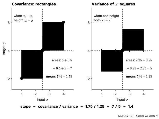
ML01.4.2-F3
The last two columns of the table as areas. Each product is a rectangle from the point of means to an example. Each squared deviation is a square of the same width. The slope is the total area of the rectangles divided by the total area of the squares.
The covariance is \(7/4 = 1.75\) and the variance is \(5/4 = 1.25\), so
Check the two balances. The predictions are \(1.9, 3.3, 4.7, 6.1\) and the residuals are \(-0.1,\ 0.3,\ -0.3,\ 0.1\). They sum to zero. Weighted by \(x\) they give \(-0.1 + 0.6 - 0.9 + 0.4 = 0\). And the loss is
against \(0.25\) for line Q and \(0.5\) for line P. No line does better.
Code
From scratch, in plain Python, following the table column by column.
x = [1.0, 2.0, 3.0, 4.0]y = [2.0, 3.0, 5.0, 6.0]n =len(x)x_bar =sum(x) / ny_bar =sum(y) / ncovariance =sum((xi - x_bar) * (yi - y_bar) for xi, yi inzip(x, y)) / nvariance =sum((xi - x_bar) **2for xi in x) / nw = covariance / varianceb = y_bar - w * x_barprint(f"means: {x_bar}, {y_bar} covariance: {covariance} variance: {variance}")print(f"slope w = {w:.4f} intercept b = {b:.4f}")
means: 2.5, 4.0   covariance: 1.75   variance: 1.25
slope w = 1.4000   intercept b = 0.5000
Now check the two equations. The partial derivatives come from the formulas of the formal section and, as a test of those formulas, from tiny nudges of each parameter.
import numpy as npx, y = np.array(x), np.array(y)def loss(w, b):return np.mean((w * x + b - y) **2)def slopes(w, b):"""The partial derivatives dL/dw and dL/db, from the formulas.""" r = w * x + b - yreturn2* np.mean(r * x), 2* np.mean(r)tidy =lambda value: round(float(value), 4) +0.0# no "-0.0" in the print-outh =1e-6for w0, b0 in [(1.0, 1.5), (w, b)]: dw, db = slopes(w0, b0) dw_nudge = (loss(w0 + h, b0) - loss(w0 - h, b0)) / (2* h) db_nudge = (loss(w0, b0 + h) - loss(w0, b0 - h)) / (2* h)print(f"w = {w0:.1f}, b = {b0:.1f}: dL/dw = {tidy(dw)} (nudge: {tidy(dw_nudge)}), "f"dL/db = {tidy(db)} (nudge: {tidy(db_nudge)}), L = {loss(w0, b0):.2f}")
w = 1.0, b = 1.5:  dL/dw = -1.0 (nudge: -1.0),  dL/db = 0.0 (nudge: 0.0),  L = 0.25
w = 1.4, b = 0.5:  dL/dw = 0.0 (nudge: 0.0),  dL/db = 0.0 (nudge: 0.0),  L = 0.05
Line Q, the first row, is flat for \(b\) but slopes downhill for \(w\): the loss would fall if \(w\) grew. At the least-squares line both slopes are zero. The libraries agree, and the last line shows a classic slip.
from sklearn.linear_model import LinearRegressionslope, intercept = np.polyfit(x, y, deg=1)model = LinearRegression().fit(x.reshape(-1, 1), y) # scikit-learn wants one column per featureprint(f"np.polyfit: w = {slope:.4f}, b = {intercept:.4f}")print(f"LinearRegression: w = {model.coef_[0]:.4f}, b = {model.intercept_:.4f}")mixed = np.cov(x, y)[0, 1] / np.var(x) # np.cov divides by n - 1, np.var by nsame = np.cov(x, y, ddof=0)[0, 1] / np.var(x) # both divide by nprint(f"mixed divisors: {mixed:.4f} same divisor: {same:.4f}")
np.polyfit:        w = 1.4000, b = 0.5000
LinearRegression:  w = 1.4000, b = 0.5000
mixed divisors: 1.8667   same divisor: 1.4000
Explore
The line fitter in lesson 1 now has an explanation. Press Show best fit there and the dashed line is the one this lesson’s formula gives. Drag a point and the line is recomputed from the new covariance and variance. Then try to beat it with the sliders: the read-out shows your loss can match it and never go below it.
Pitfalls
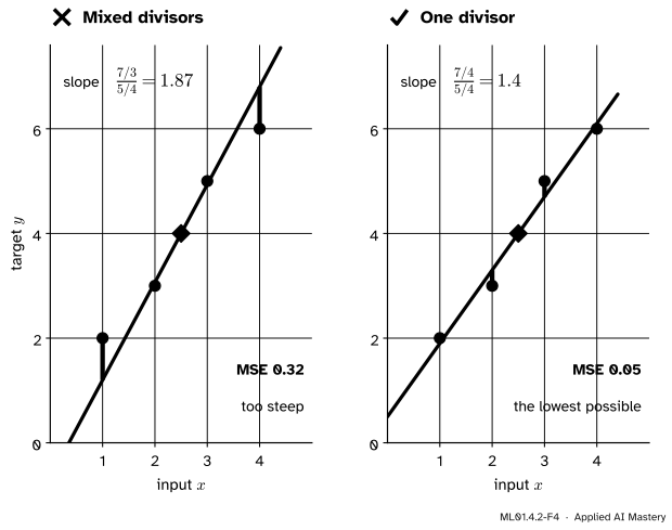
ML01.4.2-F4
Wrong beside right. Dividing the covariance by \(n - 1\) and the variance by \(n\) gives a slope that is too steep by a factor of \(4/3\). Use the same divisor in both and it cancels.
“np.cov(x, y)[0, 1] / np.var(x) is covariance over variance.”
By default np.cov divides by \(n - 1\) and np.var divides by \(n\). Mixing them multiplies the slope by \(n/(n - 1)\). With four points that turns \(1.4\) into \(1.87\) and the loss from \(0.05\) into \(0.32\). Either convention is fine for the slope, as long as the top and the bottom use the same one. Pass ddof=0 to np.cov, or ddof=1 to np.var.
“The best line goes through as many points as it can.”
The least-squares line of the four points goes through none of them. The one point it must pass through is the point of means, \((2.5, 4)\), which is not an example at all. A line through two of the points, such as line P, is perfect on those two and pays for it on the others.
“Setting the derivative to zero always finds the minimum.”
A zero slope marks a flat spot: a lowest point, a highest point, or neither. It works here because this loss is two squares plus a constant, so its only flat spot is its lowest point. Most losses in machine learning have no such guarantee, and for most the two equations cannot be solved by hand at all. That is why the next module walks downhill instead.
“Predicting \(x\) from \(y\) gives the same line, read the other way.”
It does not. Swapping the roles gives slope \(s_{xy}/s_y^2 = 1.75/2.5 = 0.7\) and intercept \(2.5 - 0.7 \cdot 4 = -0.3\), the line \(x = {0.7y - 0.3}\). Solved for \(y\) that is \(y = {1.43x + 0.43}\), not \(y = {1.4x + 0.5}\). One line makes vertical misses small and the other horizontal misses. Decide which quantity you are predicting before you fit.
Check yourself
Recall
1. What is true of the two partial derivatives of the loss at the best line?
Show answer
Both are zero: \(\pd{L}{w} = 0\) and \(\pd{L}{b} = 0\). The loss is flat in both directions.
2. Give the formulas for the best slope and the best intercept.
Show answer
The covariance of \(x\) and \(y\) over the variance of \(x\),
3. Which point does the least-squares line always pass through?
Show answer
The point of means, \((\bar{x}, \bar{y})\). That is what the equation \(w\bar{x} + b = \bar{y}\) says.
4. What do the two equations say about the residuals of the best line?
Show answer
The residuals sum to zero, \(\sum_i r_i = 0\), and so do the residuals times the inputs, \(\sum_i r_i x_i = 0\).
5. When does the slope formula have no answer?
Show answer
When every \(x_i\) is the same. The variance of \(x\) is then zero, and every line through the point of means has the same loss.
Exercises
1.★ Find the least-squares line of the three points \((1, 1)\), \((2, 3)\) and \((3, 2)\), and its mean squared error.
Show solution
The means are \(\bar{x} = 2\) and \(\bar{y} = 2\). The deviations of \(x\) are \(-1, 0, 1\) and of \(y\) are \(-1, 1, 0\). The products are \(1, 0, 0\), with sum \(1\). The squared deviations of \(x\) are \(1, 0, 1\), with sum \(2\). So \(w = 1/2 = 0.5\) and \(b = 2 - 0.5 \cdot 2 = 1\): the line is \(\hat{y} = {0.5x + 1}\).
The predictions are \(1.5, 2, 2.5\) and the residuals \(0.5, -1, 0.5\). They sum to zero, and weighted by \(x\) they give \(0.5 - 2 + 1.5 = 0\). The loss is \({(0.25 + 1 + 0.25)}/3 = 0.5\).
2.★★ Five students studied for \(2, 4, 5, 1, 3\) hours and scored \(55, 65, 80, 40, 60\) in a quiz (the study table of course P01). Find the least-squares line that predicts the score from the hours, and its mean squared error. Compare that with the loss of always predicting the mean score.
Show solution
The means are \(\bar{x} = 15/5 = 3\) hours and \(\bar{y} = 300/5 = 60\) points. The deviations of the hours are \(-1, 1, 2, -2, 0\) and of the scores \(-5, 5, 20, -20, 0\).
Products: \(5, 5, 40, 40, 0\), with sum \(90\). Squared deviations of the hours: \(1, 1, 4, 4, 0\), with sum \(10\). So \(w = 90/10 = 9\) and \(b = 60 - 9 \cdot 3 = 33\): the line is \(\hat{y} = {9x + 33}\).
The predictions are \(51, 69, 78, 42, 60\) and the residuals \(-4, 4, -2, 2, 0\). The loss is \({(16 + 16 + 4 + 4 + 0)}/5\), that is \(40/5 = 8\).
Always predicting the mean, \(60\), leaves the deviations \(-5, 5, 20, -20, 0\) as misses, and a loss of \({(25 + 25 + 400 + 400 + 0)}/5\), that is \(850/5 = 170\). The line cuts the loss from \(170\) to \(8\). Lesson 4 turns that comparison into a single number.
3.★★★ Suppose the model has no intercept: \(\hat{y} = wx\). Derive the best \(w\) by setting the derivative of the mean squared error to zero. Compute it for the four points, with its loss, and explain why the residuals no longer sum to zero.
Show solution
The loss is \(L(w) = \frac{1}{n} \sum_i (w x_i - y_i)^2\). By the chain rule,
\[
w = \frac{\overline{xy}}{\overline{x^2}} = \frac{\sum_i x_i y_i}{\sum_i x_i^2}.
\] The second derivative is \(2\,\overline{x^2} > 0\), so this is a minimum.
For the four points, \(w = 47/30 \approx 1.567\). The predictions are \(\tfrac{47}{30}, \tfrac{94}{30}, \tfrac{141}{30}, \tfrac{188}{30}\), and subtracting the targets \(\tfrac{60}{30}, \tfrac{90}{30}, \tfrac{150}{30}, \tfrac{180}{30}\) gives the residuals \(-\tfrac{13}{30},\ \tfrac{4}{30},\ -\tfrac{9}{30},\ \tfrac{8}{30}\). The loss is \(\frac{169 + 16 + 81 + 64}{900 \cdot 4} = \frac{330}{3600} = \frac{11}{120} \approx 0.092\), which is worse than the \(0.05\) of the line with an intercept.
The residuals sum to \(\tfrac{-13 + 4 - 9 + 8}{30} = -\tfrac{1}{3}\), not to zero. With one parameter there is only one equation, \(\sum_i r_i x_i = 0\), and it does hold: \(\tfrac{-13 \cdot 1 + 4 \cdot 2 - 9 \cdot 3 + 8 \cdot 4}{30} = \tfrac{-13 + 8 - 27 + 32}{30} = 0\). The equation \(\sum_i r_i = 0\) came from the derivative with respect to \(b\). Without \(b\) there is nothing to slide, so the line cannot balance its misses.
Summary card
At the best line the loss is flat for both parameters, and those two equations solve exactly.
ML01.4.2-F1
Flat in both directions.
The two equations.\(\pd{L}{b} = \frac{2}{n} \sum_i r_i = 0\) and \(\pd{L}{w} = \frac{2}{n} \sum_i r_i x_i = 0\).
Slope.\(w = s_{xy}/s_x^2\): covariance over variance. In sums, \({\sum_i (x_i - \bar{x})(y_i - \bar{y})}\) divided by \({\sum_i (x_i - \bar{x})^2}\).
Intercept.\(b = {\bar{y} - w\bar{x}}\): the line passes through \((\bar{x}, \bar{y})\).
Needs. The \(x_i\) must not all be equal, and both statistics must use the same divisor.
Sources and next steps
Sources. Each was opened and checked against this lesson on 12 November 2026.
OpenStax, Introductory Statistics 2e, Section 12.3, “The Regression Equation”. Gives the least-squares line as the one that minimises the sum of squared errors, with the slope \(b\) equal to \({\sum (x - \bar{x})(y - \bar{y})}\) divided by \({\sum (x - \bar{x})^2}\) and the intercept \(a = {\bar{y} - b\bar{x}}\), and states that “the best fit line always passes through the point \((\bar{x}, \bar{y})\)”. Its letters \(a\) and \(b\) are this course’s \(b\) and \(w\).
Tengyu Ma and Andrew Ng, CS229 Lecture Notes, Stanford University, Section 1.2, “The normal equations”. Describes the method used here: minimise the cost “by explicitly taking its derivatives” with respect to the parameters “and setting them to zero”.
Mine Çetinkaya-Rundel and Johanna Hardin, Introduction to Modern Statistics, 2nd edition, Section 7.2.3. States that the point \((\bar{x}, \bar{y})\) falls on the least-squares line and gives the slope in the equivalent form \(b_1 = \frac{s_y}{s_x} r\), with \(r\) the correlation.
NumPy 2.5 reference, numpy.cov and numpy.var. The default normalisation of cov is by \(N - 1\), and the default ddof of var is zero, so it divides by \(N\): the mismatch behind the first pitfall.
Next.ML01.4.3 Many features writes the same two equations as one matrix equation that works for any number of features.