One dataset has three jobs: fit a model, choose between models, and report how good the winner is. Learn why each job needs its own examples, how to shuffle and cut a dataset with a seed, and how scikit-learn’s train_test_split does the same.
Name the three jobs a dataset has to do (fit, choose, report) and the set that does each one.
Split a dataset from scratch by shuffling the example numbers with a seed and cutting them into three sets that do not overlap.
Choose between candidate models by their validation error and report the test error of the winner once.
Explain why the validation error of the winning model is too optimistic to report.
Make a reproducible split with scikit-learn’s train_test_split and its random_state.
In review. The maths and code on this page are checked by automated tests on every change, but an independent reader has not signed it off yet. Spot a mistake or a confusing step? Tell us.
The question
You have one dataset and three things to do with it: fit a model, choose between several models, and tell someone how good the winner is. Lesson 1 showed that the examples used to fit a model cannot score it. Can one set of held-back examples do both other jobs, or does choosing spoil them too?
From the last lesson
1. What is the training error of a lookup table whose stored inputs are all different, and why?
Show answer
Zero: it returns the stored label for every stored input, whatever the labels are.
2. Which examples is a test error measured on?
Show answer
Examples that were kept away from the model while it was built.
Intuition
A dataset has three jobs.
Fit. Set the parameters of a model.
Choose. Decide between models: which family, and how flexible.
Report. Say how well the final model will do on examples it has never met.
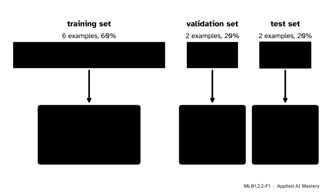
Each job spends the examples it uses. Once an example has helped to make a decision, a score on that example flatters the result. Lesson 1 was the first case: examples used to fit cannot score the fit. This lesson adds the second: examples used to choose cannot score the choice. So the dataset is cut into three sets, one for each job.
ML01.2.2-F1
Three jobs, three sets. The training set fits each candidate. The validation set chooses between them. The test set is opened once, to report on the winner.
The training set is the largest, because fitting needs the most examples. The validation set and the test set are smaller. The test set has one rule of its own: nothing may be decided by looking at it.
Build it up
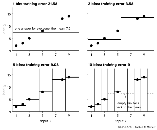
Step 1. A dial for flexibility. Choosing needs candidates. Here is a family that runs from “one answer for everyone” to the lookup table of lesson 1. Cut the range of the input into equal bins. Store one answer per bin: the mean label of the training examples that fall in it. A bin with no training example answers with the mean of all the training labels.
ML01.2.2-F3
A table with 1, 2, 5 and 10 bins, fitted to the same six training points. With one bin it is a single number. With ten it is a lookup table.
The number of bins is not set by fitting. You pick it first, and fitting then fills in the answers. A setting of this kind is a hyperparameter. The stored answers are the parameters (lesson ML01.1.3).
Step 2. Training error cannot choose the number of bins. Read the titles of the four panels: \(21.58\), \(3.58\), \(0.08\), \(0\). The training error votes for the lookup table every time.
Step 3. So choose with examples that were not used to fit. Fit every candidate on the training set, score each on held-out examples, and keep the one with the lowest score. The held-out examples used for this are the validation set.
Step 4. The winner’s validation score is now spent. The winner was picked because its validation error was the lowest. Some of that is skill and some is luck with these particular validation examples. For an honest number, score the winner on a third set that played no part in fitting or choosing. That is the test set.
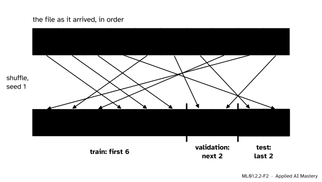
Step 5. Shuffle, then cut. Files often arrive in an order: sorted by date, by size, or by label. Cutting such a file as it stands gives sets that differ from each other. So shuffle the example numbers first, then cut.
ML01.2.2-F2
Ten example numbers are shuffled, and the shuffled row is cut after the sixth and eighth places.
A computer’s shuffle is decided by a number called the seed. The same seed gives the same shuffle every time, so anyone can make the split again.
The formal statement
NoteDefinition: a three-way split
Number the examples \(1, \dots, n\). A split sorts these numbers into three sets, train, validation and test, so that every number is in exactly one of them. Their sizes add up: \(n_{\text{train}} + n_{\text{val}} + n_{\text{test}} = n\). Each set has its own error, the same formula over different examples:
Fit. For each candidate, choose its parameters to make \(L_{\text{train}}\) small.
Choose. Keep the fitted candidate with the smallest \(L_{\text{val}}\).
Report. Compute \(L_{\text{test}}\) for that one candidate, once.
Result 1: splitting a bin never raises the training error. Take one bin \(B\) of a table and split it into two smaller bins, \(B_1\) and \(B_2\). Before the split, every training example in \(B\) got the answer \(\bar{y}_B\), the mean of the labels in \(B\). After it, an example in \(B_1\) gets \(\bar{y}_1\), the mean of the labels in \(B_1\). The mean of a group is the single answer with the smallest total squared error for that group (lesson 1, deeper block), so
Add the two lines: the total squared error in \(B\) after the split is no more than before it. No other bin changed, so \(L_{\text{train}}\) did not rise. Keep splitting until every training input has a bin of its own, and the training error reaches \(0\). This is why training error cannot do the choosing: it always prefers the finest table.
Result 2: the winner’s validation error is optimistic. Suppose there are \(K\) fitted candidates, and write \(V_k\) for the validation error of candidate \(k\). A different draw of validation examples would give different values, so each \(V_k\) is a random number, whose average \(\E[V_k]\) is the generalisation error of candidate \(k\). The winner’s score is the smallest, \(\min_j V_j\). For every \(k\),
So on average the lowest validation error is no higher than the generalisation error of the best candidate, and the winner can be no better than that: the winning score tends to promise more than the winner delivers. The test set took no part in choosing, so its error has no such lean.
How big should each set be? Common choices give each held-back set 10 to 25 percent of the data, such as 60/20/20 or 80/10/10. scikit-learn’s default test share is 25 percent, and Goodfellow, Bengio and Courville describe validating on about 20 percent of the training data. What matters is the number of held-back examples, as the next lesson shows.
Worked example
Split ten examples 6/2/2, choose the number of bins, and report.
The data are the course’s four points and six more, made up to continue their pattern: inputs \(x = 1, 2, \dots, 10\) and labels \(y = 2, 3, 5, 6, 8, 9, 11, 13, 14, 15\).
Split. A shuffle with seed 1 puts the inputs in the order \(9, 5, 8, 1, 2, 3, 6, 10, 7, 4\). The first six are the training set, the next two (\(x = 6\) and \(10\)) the validation set, and the last two (\(x = 7\) and \(4\)) the test set.
Fit. The six training examples are \((9, 14)\), \((5, 8)\), \((8, 13)\), \((1, 2)\), \((2, 3)\) and \((3, 5)\). Take the table with 5 bins, each two inputs wide.
Inputs in the bin
Training labels in it
Stored answer
\(1, 2\)
\(2,\ 3\)
\(2.5\)
\(3, 4\)
\(5\)
\(5\)
\(5, 6\)
\(8\)
\(8\)
\(7, 8\)
\(13\)
\(13\)
\(9, 10\)
\(14\)
\(14\)
Only the first bin holds two examples, and each is \(0.5\) away from the stored \(2.5\). So the training error is \({(0.25 + 0.25 + 0 + 0 + 0 + 0)}/6 = 0.08\).
Choose. Score the 5-bin table on the validation examples \((6, 9)\) and \((10, 15)\). The input \(6\) falls in the bin that answers \(8\), and \(10\) in the bin that answers \(14\): \(L_{\text{val}} = {\big((8 - 9)^2 + (14 - 15)^2\big)}/2 = 1\).
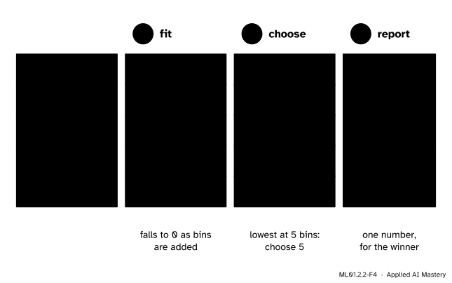
The other candidates go the same way. With 1 bin the answer is always the training mean, \(45/6 = 7.5\), so \(L_{\text{val}} = {\big((7.5 - 9)^2 + (7.5 - 15)^2\big)}/2 = {(2.25 + 56.25)}/2 = 29.25\). With 2 bins the answers are \(4.5\) for inputs up to \(5\) and \(13.5\) above, both validation inputs get \(13.5\), and \(L_{\text{val}} = {(20.25 + 2.25)}/2 = 11.25\). With 10 bins neither \(6\) nor \(10\) was seen in training, both get the fallback \(7.5\), and \(L_{\text{val}} = 29.25\) again.
ML01.2.2-F4
The whole routine as one table. Training error would choose 10 bins. Validation error chooses 5.
The lowest validation error is \(1\), so the choice is 5 bins.
Report. Now, and only now, open the test set: \((7, 11)\) and \((4, 6)\). The input \(7\) gets \(13\) and the input \(4\) gets \(5\), so \(L_{\text{test}} = {\big((13 - 11)^2 + (5 - 6)^2\big)}/2 = 2.5\).
The number to report is \(2.5\), not \(1\): the winner’s validation error was the more flattering, as Result 2 says it tends to be. Two points prove nothing, though. The next lesson measures how much such scores wobble.
Code
A split from scratch is a shuffle and two cuts.
import numpy as npdef split(n, n_val, n_test, seed):"""Shuffle the example numbers 0..n-1 with a seed, then cut: train, validation, test.""" order = np.random.default_rng(seed).permutation(n) n_train = n - n_val - n_testreturn order[:n_train], order[n_train:n_train + n_val], order[n_train + n_val:]x = np.arange(1, 11) # ten inputs, 1 to 10y = np.array([2.0, 3, 5, 6, 8, 9, 11, 13, 14, 15]) # the four points and six moretrain, val, test = split(len(x), n_val=2, n_test=2, seed=1)print("train x:", x[train], " validation x:", x[val], " test x:", x[test])
def mse(y_hat, y):return np.mean((y_hat - y) **2)def fit_table(keys, y):"""One stored answer per bin: the mean label of the training examples in that bin.""" answers = {int(k): y[keys == k].mean() for k in np.unique(keys)}return answers, y.mean() # the mean is the fallback for an empty bindef predict_table(model, keys): answers, fallback = modelreturn np.array([answers.get(int(k), fallback) for k in keys])results = {}for bins in [1, 2, 5, 10]: keys = (x -1) * bins //10# the bin that each input falls in model = fit_table(keys[train], y[train]) # FIT: training examples only results[bins] = [mse(predict_table(model, keys[part]), y[part]) for part in (train, val, test)]print(f"{bins:2d} bins training {results[bins][0]:5.2f} validation {results[bins][1]:5.2f}")best =min(results, key=lambda bins: results[bins][1]) # CHOOSE: lowest validation errorprint(f"chosen: {best} bins. REPORT: test error {results[best][2]:.2f}")
 1 bins   training 21.58   validation 29.25
 2 bins   training  3.58   validation 11.25
 5 bins   training  0.08   validation  1.00
10 bins   training  0.00   validation 29.25
chosen: 5 bins.  REPORT: test error 2.50
The numbers match the worked example. Now real data. The diabetes dataset that ships with scikit-learn has 442 patients, ten features measured at a first visit, and a label: a measure of how far the disease had progressed a year later. We use one feature, the body mass index (BMI), and add a line to the candidates.
from sklearn.datasets import load_diabetesdata = load_diabetes(scaled=False) # 442 patients, 10 features eachbmi, progression = data.data[:, 2], data.target # one feature (the BMI) and the labeltenths = np.round(bmi *10).astype(int) # BMI is recorded to 0.1, so 32.1 becomes 321train, val, test = split(len(bmi), n_val=89, n_test=89, seed=0)print("sizes:", len(train), len(val), len(test))scores = {}w, b = np.polyfit(bmi[train], progression[train], deg=1) # the best-fitting line, training set onlyscores["line"] = [mse(w * bmi[part] + b, progression[part]) for part in (train, val, test)]for bins in [1, 5, 25, 250]: keys = (tenths -180) * bins //250# equal bins from BMI 18.0 to 43.0 model = fit_table(keys[train], progression[train]) scores[f"{bins} bins"] = [mse(predict_table(model, keys[part]), progression[part])for part in (train, val, test)]for name, (training, validation, _) in scores.items():print(f"{name:9} training {training:5.0f} validation {validation:5.0f}")best =min(scores, key=lambda name: scores[name][1])print(f"chosen: {best}. test error, reported once: {scores[best][2]:.0f}")
sizes: 264 89 89
line      training  3728   validation  3872
1 bins    training  6148   validation  6243
5 bins    training  3814   validation  4540
25 bins   training  3520   validation  3977
250 bins  training  1772   validation  6930
chosen: line.  test error, reported once: 4418
With 250 bins each recorded BMI value has its own bin, so that table is a lookup table. Its training error is the lowest, \(1{,}772\), and its validation error the highest, \(6{,}930\). The line has the lowest validation error, \(3{,}872\), so it is chosen, and its test error is \(4{,}418\).
Last, the library. train_test_split shuffles and makes one cut, so a three-way split takes two calls. Its random_state is the seed.
from sklearn.model_selection import train_test_splitX = bmi.reshape(-1, 1) # scikit-learn wants a columnX_rest, X_test, y_rest, y_test = train_test_split(X, progression, test_size=89, random_state=0)X_train, X_val, y_train, y_val = train_test_split(X_rest, y_rest, test_size=89, random_state=0)print("sizes:", len(X_train), len(X_val), len(X_test))again = train_test_split(X, progression, test_size=89, random_state=0)print("same seed, same test set:", np.array_equal(again[1], X_test))print("default test share:", round(len(train_test_split(X, progression, random_state=0)[1]) /len(X), 2))
sizes: 264 89 89
same seed, same test set: True
default test share: 0.25
test_size may be a count, as here, or a share such as 0.2. Shuffling is on by default. For classification, stratify keeps the share of each class the same in every set.
Explore
This module’s interactive, the split explorer, is in lesson 3. There you set the number of bins of this lesson’s table, reshuffle the split, and watch both errors move.
Pitfalls
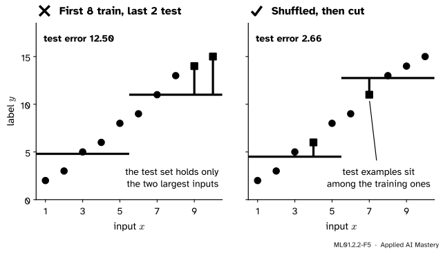
ML01.2.2-F5
Wrong beside right, for a file sorted by input.
“I will take the first 80 percent for training and the rest for testing.”
Only if the file is in random order, and you rarely know that. In the figure the file is sorted: the test set holds only the largest inputs, and the same 2-bin table scores \(12.50\) on it, against \(2.66\) after a shuffle. The exception is data ordered in time, which lesson 4 covers.
“Two sets are enough: I will choose the model on the test set.”
Then that set is a validation set, whatever you call it, and you have no test set. By Result 2, the score of the model chosen with it is optimistic.
“The test set says another candidate was better, so I will switch to that one.”
On the diabetes data the line was chosen and scored \(4{,}418\) on the test set. The 5-bin table, which lost on validation, scores \(4{,}247\) there. Switching would be choosing with the test set, and \(4{,}247\) would no longer be an honest report.
Check yourself
Recall
1. What are the three jobs of a dataset, and which set does each?
Show answer
Fit, with the training set. Choose, with the validation set. Report, with the test set.
2. What is a hyperparameter? Give the example from this lesson.
Show answer
A setting fixed before fitting, not by it, such as the number of bins. The stored answers in the bins are the parameters.
3. Why can the training error not be used to choose the number of bins?
Show answer
Splitting a bin never raises the training error, so it always prefers the finest table: the lookup table.
4. Why is the validation error of the chosen model not a fair report of how good it is?
Show answer
It was chosen for having the lowest validation error, and part of that is luck. The lowest of several noisy scores tends to be too low.
5. What does a seed do, and why record it?
Show answer
It fixes the shuffle: the same seed gives the same split every time, so the results can be reproduced.
Exercises
1.★ A dataset has 1,000 examples and is split 70/15/15. How many examples are in each set? A shuffle of the numbers 1 to 8 gives \(3, 7, 1, 8, 5, 2, 6, 4\), and the split is 4/2/2 in that order. List the three sets.
Show solution
The sizes are \(700\), \(150\) and \(150\).
Cutting after the fourth and sixth places gives the training set \(\{3, 7, 1, 8\}\), the validation set \(\{5, 2\}\) and the test set \(\{6, 4\}\).
2.★★ In the worked example, swap the roles of the last two sets: let \(x = 7\) and \(x = 4\) be the validation set and \(x = 6\) and \(x = 10\) the test set. The training set is unchanged. Which number of bins is chosen now, and what is reported?
Show solution
The fitted tables are unchanged, because the training set is. Their errors on the new validation set, \((7, 11)\) and \((4, 6)\):
1 bin: both get \(7.5\), so \({\big((7.5 - 11)^2 + (7.5 - 6)^2\big)}/2 = {(12.25 + 2.25)}/2 = 7.25\).
2 bins: \(7\) gets \(13.5\) and \(4\) gets \(4.5\), so \({(6.25 + 2.25)}/2 = 4.25\).
5 bins: \(7\) gets \(13\) and \(4\) gets \(5\), so \({(4 + 1)}/2 = 2.5\).
10 bins: neither input was seen, both get \(7.5\), so \(7.25\).
The lowest is \(2.5\), so 5 bins is chosen again. Its error on the new test set, \((6, 9)\) and \((10, 15)\), is \(1\). This time the test error is the lower of the two: Result 2 is about the average.
3.★★★ A shuffle makes every ordering of the \(n\) example numbers equally likely, and the last \(n_{\text{test}}\) places are the test set. Find the probability that two given examples both land in the test set, and evaluate it for the 6/2/2 split of ten examples.
Show solution
Every ordering is equally likely, so the first example is equally likely to be in each of the \(n\) places, and it is in a test place with probability \(n_{\text{test}}/n\). Given that, \(n - 1\) places remain for the second, all equally likely, and \(n_{\text{test}} - 1\) of them are test places. Multiply the two:
\[
\begin{aligned}
&\Prob(\text{both in the test set}) \\
&\quad = \frac{n_{\text{test}}}{n} \cdot \frac{n_{\text{test}} - 1}{n - 1} .
\end{aligned}
\]
For \(n = 10\) and \(n_{\text{test}} = 2\) this is \(\frac{2}{10} \cdot \frac{1}{9} = \frac{1}{45} \approx 0.022\).
Summary card
Three jobs, three sets: fit on the training set, choose on the validation set, report on the test set, once.
ML01.2.2-F1
Fit, choose, report.
A split. Shuffle the example numbers with a seed, then cut. Every example is in exactly one set.
Fit. Parameters come from \(L_{\text{train}}\). Splitting a bin never raises it, so it cannot choose the flexibility.
Choose. Hyperparameters come from \(L_{\text{val}}\). The winner’s score is optimistic: \(\E[\min_j V_j] \le \min_k \E[V_k]\).
Report.\(L_{\text{test}}\) of the winner, computed once and never used to decide anything.
Sources and next steps
Sources. Each was opened and checked against this lesson on 12 November 2026.
Ian Goodfellow, Yoshua Bengio and Aaron Courville, Deep Learning, MIT Press, 2016, Section 5.3. Defines hyperparameters and the validation set, states that test examples must not be used in any way to make choices about the model, gives the 80 and 20 percent split, and notes that the validation error underestimates the generalisation error.
scikit-learn developers, Cross-validation: evaluating estimator performance, User Guide, Section 3.1 (version 1.9.1). Tuning settings against the test set lets knowledge of it leak into the model, so a validation set is held out and the test set is kept for the final evaluation.
scikit-learn developers, train_test_split, API reference (version 1.9.1). test_size is a share or a count and defaults to 0.25, shuffle defaults to true, random_state makes the output reproducible, stratify splits by class.
scikit-learn developers, Diabetes dataset, User Guide, Section 9.1.2. 442 patients, ten baseline variables including the body mass index, and a quantitative measure of disease progression one year after baseline.
Next.ML01.2.3 The generalization gap measures the distance between training error and test error, and asks how far a test error can be trusted.