Three kinds of model, linear regression, k-nearest neighbours and the lasso, are tuned and scored on the same five folds. Their scores come with standard errors, the differences are compared fold by fold, and a rule fixed in advance picks the winner.
Score several pipelines on the same folds and report each score with its standard error.
Tune one setting of a model by cross-validation and read its tuning curve.
Compare two models fold by fold, and explain why the paired difference is steadier than either score.
Apply the one-standard-error rule to choose the simplest model that is as good as the best.
In review. The maths and code on this page are checked by automated tests on every change, but an independent reader has not signed it off yet. Spot a mistake or a confusing step? Tell us.
The question
Three kinds of model are tried on the 353 working patients. After tuning, their cross-validated errors are \(45.1\), \(45.5\) and \(46.3\). Which one should the clinic use? Before answering, ask a sharper question: is a gap of one point a real difference between models, or is it the luck of which patients fell into which fold?
From the last lesson
1. From which rows does a preparation step learn its numbers?
Show answer
From the training rows only. Held-out rows are transformed with the stored numbers.
2. Ten columns of pure noise scored \(55.61\), better than the baseline’s \(64.83\). What had gone wrong?
Show answer
The ten columns were chosen using all the rows, before the folds were cut, so the choice had seen every held-out fold. Chosen inside each fold they scored \(70.44\).
Intuition
A cross-validated score is a measurement, and a measurement has an error bar. With five folds you have five numbers per model. Their mean is the score. Their spread says how far that mean could have landed elsewhere. A fair comparison shows both.
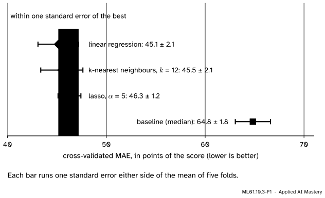
ML01.10.3-F1
The result of this lesson. The three models are about twenty points better than the baseline, and all three lie within one standard error of the best. The gaps between them are smaller than their error bars.
Do the models beat the baseline? Yes, by about ten standard errors. Which model is best? The data cannot say. When the data cannot say, something else must decide, and it must have been agreed beforehand. Lesson 1 agreed it: take the simplest model within one standard error of the best.
Build it up
Step 1. Same folds for everyone. Every candidate is fitted on the same four folds and scored on the same fifth, five times. A fold of hard patients is then hard for every model and cannot favour one of them.
Step 2. Three candidates, each in a pipeline.
Linear regression on the ten features (ML01.4.3). It has nothing to tune.
\(k\)-nearest neighbours on standardised features (ML01.3.4). One setting: \(k\).
The lasso on standardised features (ML01.9.2): linear regression with a price on the sum of the absolute weights. One setting: the price. scikit-learn calls it alpha, written \(\alpha\) here. It is half the \(\lambda\) of ML01.9.2, because scikit-learn halves the squared error.
Step 3. Tune each setting by cross-validation. Try a grid of values. For each value run the five folds and average. Plot the average against the setting: this is the tuning curve.
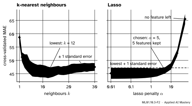
ML01.10.3-F2
The two tuning curves, each with a band of one standard error. For \(k\)-NN the curve has a bottom, at \(k = 12\). For the lasso it is flat and then climbs: the lowest point is the smallest penalty tried.
Step 4. Read the curves. For \(k\)-NN the lowest error is at \(k = 12\). Smaller \(k\) follows noise and larger \(k\) blurs, as in ML01.3.2. For the lasso the error is lowest at the smallest\(\alpha\) on the grid. That is a finding: with 353 patients and ten features, plain linear regression is not overfitting, and a penalty has nothing to cure.
Step 5. Use the flat part. The lasso curve barely moves until \(\alpha = 2\). Along that flat stretch the model gets simpler, because the lasso sets weights to exactly zero, and its score stays inside the band. The one-standard-error rule takes the simplest setting whose score is no more than one standard error above the lowest. Here that is \(\alpha = 5\), which keeps five features of the ten.
Step 6. Compare fold by fold. To compare two models, subtract their scores fold by fold and look at the five differences. The shared difficulty of each fold cancels.
The formal statement
NoteDefinition: cross-validated score and its standard error
Let \(s_1, \dots, s_k\) be the scores of one pipeline on \(k\) held-out folds. Its cross-validated score is their mean \(\bar{s}\). The standard error of that mean is
The standard deviation divides by \(k - 1\), the usual choice for a handful of values. Three results turn these numbers into a decision.
Result 1: the difference of two scores is the mean of the fold differences. Let model A score \(a_j\) and model B score \(b_j\) on fold \(j\), and write \(d_j = {b_j - a_j}\). Then
So the gap between two models is itself a mean of \(k\) numbers, and its standard error is the standard deviation of the \(d_j\) divided by \(\sqrt{k}\).
Result 2: differences are steadier when the scores move together. Write \(\text{Var}\) for the variance, \(u_j = {b_j - \bar{b}}\) and \(v_j = {a_j - \bar{a}}\). By Result 1, \({d_j - \bar{d}} = {u_j - v_j}\). Expand the square:
where \(\text{Cov}(a, b) = \frac{1}{k-1}\sum_j v_j u_j\) is the covariance, the cross term of the square. When a fold that is hard for A is also hard for B, the covariance is positive, and the differences vary less than the two scores would suggest. This is what using the same folds buys.
Result 3: the one-standard-error rule. Among the settings of a model, let \(\bar{s}^{*}\) be the lowest cross-validated score and \(\text{SE}^{*}\) its standard error. Choose the simplest setting whose score satisfies
\[
\bar{s} \le \bar{s}^{*} + \text{SE}^{*} .
\]
For the lasso, “simplest” means the largest \(\alpha\), which here keeps the fewest features. The rule is a convention, not a theorem. It says: do not pay in complexity for an improvement you cannot tell from noise.
Go deeper: how far to trust a standard error from five folds
Only roughly. The formula for the standard error of a mean assumes independent values. Fold scores are not independent: any two training sets share three of their four folds, so the five models are nearly the same model. Bengio and Grandvalet proved that no estimate of the variance of a score from \(k\) folds is unbiased for every kind of data, and showed that a simple estimate like this one can be far too small. Read “\(\pm 2.1\)” as “at least about 2”. The three models are then even harder to tell apart.
Also, the \(k\)-NN score of \(45.50\) is the lowest of thirty tuning scores, and a lowest-of-many is biased low (ML01.2.2). Its honest value is a little higher. Only rows that played no part in any choice can settle it: the test set, in the next lesson.
Worked example
Is \(k\)-NN worse than linear regression? Their fold scores, to one decimal:
Fold \(j\)
Linear \(a_j\)
\(k\)-NN \(b_j\)
\(d_j = {b_j - a_j}\)
1
\(52.8\)
\(48.6\)
\(-4.2\)
2
\(44.6\)
\(40.5\)
\(-4.1\)
3
\(41.1\)
\(41.4\)
\(0.3\)
4
\(45.2\)
\(51.8\)
\(6.6\)
5
\(42.0\)
\(45.3\)
\(3.3\)
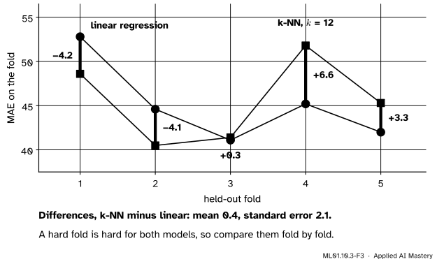
ML01.10.3-F3
The same five folds, two models. Each purple bar is one difference \(d_j\).
The scores. The linear scores add up to \(225.7\), so \(\bar{a} = 45.14\). Their deviations from the mean are \(7.66, -0.54, -4.04, 0.06, -3.14\), with squares adding up to \(85.15\). So \(\text{sd} = \sqrt{85.15/4} = 4.61\) and \(\text{SE} = 4.61/\sqrt{5} = 2.06\). The same steps for \(k\)-NN give \(\bar{b} = 45.52\) and \(\text{SE} = 2.13\).
The difference. The \(d_j\) add up to \(1.9\), so \(\bar{d} = 0.38\), which is \(45.52 - 45.14\) as Result 1 says. Their deviations are \(-4.58, -4.48, -0.08, 6.22, 2.92\), with squares adding up to \(88.27\). So \(\text{sd} = \sqrt{88.27/4} = 4.70\) and \(\text{SE} = 4.70/\sqrt{5} = 2.10\).
The gap is \({0.38 \pm 2.10}\). It is a fifth of its own standard error. \(k\)-NN won two folds and lost three. There is no evidence here that either model is better.
Check Result 2. The variances are \(85.15/4 = 21.29\) and \(22.79\), and the covariance is \(11.00\). So \(\text{Var}(d) = {21.29 + 22.79 - 2 \times 11.00} = 22.08\), which is \(4.70^2\) up to rounding. Had the two models been scored on different folds, the covariance term would be missing and the standard error of the gap would be \(\sqrt{(21.29 + 22.79)/5} = 2.97\) instead of \(2.10\).
The one-standard-error rule for the lasso. The lowest score is \(45.15\) at \(\alpha = 0.01\), with standard error \(2.05\). The limit is \({45.15 + 2.05} = 47.20\).
\(\alpha\)
Score
Features kept
Inside the limit?
\(2\)
\(45.46\)
7
yes
\(5\)
\(46.27\)
5
yes
\(10\)
\(47.83\)
4
no
The largest \(\alpha\) inside the limit is \(5\).
Code
From scratch: a method is a function that takes training rows and returns predictions for new rows. One loop scores any method on the five folds.
import numpy as npfrom sklearn.datasets import load_diabetesfrom sklearn.model_selection import train_test_splitdata = load_diabetes(scaled=False)X_work, X_test, y_work, y_test = train_test_split(data.data, data.target, test_size=89, random_state=10)folds = np.array_split(np.arange(len(y_work)), 5) # the five folds of lessons 1 and 2def median(X_train, y_train, X_new):return np.full(len(X_new), np.median(y_train))def linear(X_train, y_train, X_new): A = np.column_stack([X_train, np.ones(len(X_train))]) # a column of ones for the bias (ML01.4.3) w = np.linalg.lstsq(A, y_train, rcond=None)[0]return np.column_stack([X_new, np.ones(len(X_new))]) @ wdef knn(k):def predict(X_train, y_train, X_new): mean, sd = X_train.mean(axis=0), X_train.std(axis=0) # learned from the training rows Z_train, Z_new = (X_train - mean) / sd, (X_new - mean) / sd distance = np.sqrt(((Z_new[:, None, :] - Z_train[None, :, :]) **2).sum(axis=2)) nearest = np.argsort(distance, axis=1, kind="stable")[:, :k]return y_train[nearest].mean(axis=1) # the mean target of the k nearest (ML01.3.4)return predictdef cv_scores(method):"""The MAE of a method on each fold, fitted each time on the other four.""" scores = []for held in folds: train = np.setdiff1d(np.arange(len(y_work)), held) y_hat = method(X_work[train], y_work[train], X_work[held]) scores.append(np.mean(np.abs(y_work[held] - y_hat)))return np.array(scores)def se(values):return values.std(ddof=1) / np.sqrt(len(values))s_base, s_lin, s_knn = cv_scores(median), cv_scores(linear), cv_scores(knn(12))for name, s in [("baseline (median)", s_base), ("linear regression", s_lin), ("k-NN, k = 12", s_knn)]:print(f"{name:18} folds {np.round(s, 1)} mean {s.mean():.2f} se {se(s):.2f}")gap = s_knn - s_linprint(f"k-NN minus linear: {np.round(gap, 1)} mean {gap.mean():.2f} se {se(gap):.2f}")print(f"se of the gap if the folds were not shared: {np.sqrt(se(s_knn) **2+ se(s_lin) **2):.2f}")
baseline (median)  folds [66.  67.5 58.8 68.7 63.1]   mean 64.83   se 1.78
linear regression  folds [52.8 44.6 41.1 45.2 42. ]   mean 45.14   se 2.06
k-NN, k = 12       folds [48.6 40.5 41.4 51.8 45.3]   mean 45.50   se 2.13
k-NN minus linear: [-4.2 -4.1  0.3  6.6  3.2]   mean 0.36   se 2.09
se of the gap if the folds were not shared: 2.96
With every decimal kept, the gap is \({0.36 \pm 2.09}\). The worked example rounded the fold scores first.
The library does the tuning. GridSearchCV (ML01.9.4) takes a pipeline and a grid, runs the five folds for every value, and keeps each fold’s score. The name of a setting inside a pipeline is the step’s name, two underscores, and the setting.
from sklearn.linear_model import Lassofrom sklearn.model_selection import GridSearchCV, KFoldfrom sklearn.neighbors import KNeighborsRegressorfrom sklearn.pipeline import make_pipelinefrom sklearn.preprocessing import StandardScalerdef search(model, grid): pipeline = make_pipeline(StandardScaler(), model) found = GridSearchCV(pipeline, grid, cv=KFold(n_splits=5), scoring="neg_mean_absolute_error").fit(X_work, y_work) per_fold =-np.array([found.cv_results_[f"split{j}_test_score"] for j inrange(5)])return per_fold # one row per fold, one column per settingks =list(range(1, 31))knn_folds = search(KNeighborsRegressor(), {"kneighborsregressor__n_neighbors": ks})k_mean = knn_folds.mean(axis=0)print("k-NN, lowest score:", round(k_mean.min(), 2), "at k =", ks[k_mean.argmin()])print("k = 1, 5, 12, 30:", np.round(k_mean[[0, 4, 11, 29]], 2))alphas = [0.01, 0.02, 0.05, 0.1, 0.2, 0.5, 1, 2, 5, 10, 20, 50]lasso_folds = search(Lasso(), {"lasso__alpha": alphas})a_mean, a_se = lasso_folds.mean(axis=0), lasso_folds.std(axis=0, ddof=1) / np.sqrt(5)limit = a_mean.min() + a_se[a_mean.argmin()]pick =max(j for j inrange(len(alphas)) if a_mean[j] <= limit) # the strongest penalty inside the limitprint("lasso scores:", np.round(a_mean, 2))print(f"lowest {a_mean.min():.2f} at alpha = {alphas[a_mean.argmin()]}, limit {limit:.2f}, chosen alpha = {alphas[pick]}")
s_lasso = lasso_folds[:, pick]chosen = make_pipeline(StandardScaler(), Lasso(alpha=alphas[pick])).fit(X_work, y_work)weights = {name: round(float(w), 2) for name, w inzip(data.feature_names, chosen[-1].coef_) if w !=0}print("features kept:", weights)results = {"baseline (median)": s_base, "linear regression": s_lin, "k-NN, k = 12": s_knn, "lasso, alpha = 5": s_lasso}for name, s in results.items(): against = s - s_linprint(f"{name:18}{s.mean():6.2f} +/- {se(s):.2f} minus linear: {against.mean():6.2f} +/- {se(against):.2f}")best =min(results, key=lambda name: results[name].mean())limit_all = results[best].mean() + se(results[best])inside = [name for name, s in results.items() if s.mean() <= limit_all]print(f"best: {best}; limit {limit_all:.2f}; inside the limit: {inside}")
features kept: {'sex': -1.44, 'bmi': 23.57, 'bp': 10.32, 's3': -7.91, 's5': 20.59}
baseline (median)   64.83 +/- 1.78    minus linear:  19.69 +/- 1.91
linear regression   45.14 +/- 2.06    minus linear:   0.00 +/- 0.00
k-NN, k = 12        45.50 +/- 2.13    minus linear:   0.36 +/- 2.09
lasso, alpha = 5    46.27 +/- 1.16    minus linear:   1.13 +/- 1.13
best: linear regression; limit 47.20; inside the limit: ['linear regression', 'k-NN, k = 12', 'lasso, alpha = 5']
The lasso keeps bmi, s5, bp, s3 and sex. Their weights are in points of the score per standard deviation of the feature, so they can be compared: body mass index and s5 matter most. The paper that published this table found these five entering in the same order.
Linear regression has the lowest score, \(45.14\), so the limit is \({45.14 + 2.06} = 47.20\). All three models are inside it. The simplest, by the rule agreed in lesson 1, is the lasso: five measurements instead of ten, at a cost of \({1.13 \pm 1.13}\) points. The lasso with \(\alpha = 5\) goes forward.
Explore
ML01.10-X1
Project board
Build a pipeline stage by stage. Start at stage 2: press Standardised and watch the \(k\)-NN curve drop below the grey curve it leaves behind. Then switch to the Linear model and try the same button: its score, \(45.14\), does not move.
Things to try.
With \(k\)-NN, press Best validation score. Standardised, it is \(45.50\) at \(k = 12\).
Choose Linear model and Lasso, and slide \(\alpha\) up from \(0\). The read-out counts the features kept. At \(\alpha = 5\) it says \(46.27\), inside one standard error of the lowest. (For ridge, scikit-learn’s alpha is \(n\) times ML01.9’s \(\lambda\).)
Only now press Open the test set. Then move a slider and watch the read-out count the pipelines whose test score you have seen. The best test score among them is no longer an honest estimate.
Pitfalls
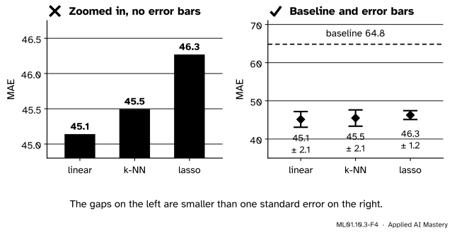
ML01.10.3-F4
Wrong beside right. The same three numbers. A zoomed axis turns one point into a cliff. Error bars and the baseline put it back in proportion.
“45.1 is lower than 46.3, so linear regression is the better model.”
Not on this evidence: the gap is \(1.13\) with a standard error of \(1.13\). A table of scores without error bars invites a ranking the data do not support. Report the standard error, and compare fold by fold.
“The best setting is at the edge of my grid. Fine.”
An edge means the curve may still be falling beyond it. Widen the grid, or work out what the edge means. Here the lasso’s lowest score is at the smallest \(\alpha\), and beyond that edge lies \(\alpha = 0\): plain linear regression, which is already a candidate.
“I tuned my favourite model and compared it with the others at their defaults.”
Then the comparison measures effort. \(k\)-NN at scikit-learn’s default, \(k = 5\), scores \(47.41\); tuned, \(45.50\). Give every candidate the same care.
Check yourself
Recall
1. How is the standard error of a cross-validated score computed from the fold scores?
Show answer
Take the standard deviation of the \(k\) fold scores (dividing by \(k - 1\)) and divide it by \(\sqrt{k}\).
2. Why score every candidate on the same folds?
Show answer
A hard fold is then hard for every model. The fold-by-fold differences cancel that shared difficulty, so the gap between two models is measured more steadily.
3. State the one-standard-error rule.
Show answer
Choose the simplest setting whose cross-validated score is no more than one standard error above the lowest score.
4. The lasso’s lowest score was at the smallest \(\alpha\) tried. What does that say?
Show answer
That the penalty does not improve the predictions here: plain linear regression is not overfitting. The penalty can still buy a simpler model at almost no cost.
5. Which model goes forward, and why that one?
Show answer
The lasso with \(\alpha = 5\). All three models are within one standard error of the best, and it is the simplest: it uses five features.
Exercises
1.★ A model scores \(30, 34, 29, 35, 32\) on five folds. Find its cross-validated score and standard error.
Show solution
The mean is \(160/5 = 32\). The deviations are \(-2, 2, -3, 3, 0\), with squares \(4, 4, 9, 9, 0\) adding up to \(26\). So \(\text{sd} = \sqrt{26/4} = 2.55\) and \(\text{SE} = 2.55/\sqrt{5} = 1.14\). The score is \({32 \pm 1.14}\).
2.★★ A second model scores \(31, 36, 30, 37, 33\) on the same five folds. (a) Find the mean and the standard error of the fold-by-fold differences, second minus first. (b) Is the second model worse? (c) What would the standard error of the gap be if you ignored the pairing?
Show solution
(a) The differences are \(1, 2, 1, 2, 1\), with mean \(7/5 = 1.4\). Their deviations are \(-0.4, 0.6, -0.4, 0.6, -0.4\), with squares adding up to \(0.16 + 0.36 + 0.16 + 0.36 + 0.16 = 1.2\). So \(\text{sd} = \sqrt{1.2/4} = 0.55\) and \(\text{SE} = 0.55/\sqrt{5} = 0.24\).
(b) Yes. The gap is \({1.4 \pm 0.24}\), nearly six standard errors, and the second model lost every fold.
(c) The second model has mean \(33.4\) and deviations \(-2.4, 2.6, -3.4, 3.6, -0.4\), with squares adding up to \(37.2\), so its variance is \(9.3\). The first model’s variance is \(26/4 = 6.5\). Ignoring the pairing gives \(\sqrt{(6.5 + 9.3)/5} = 1.78\), and a gap of \({1.4 \pm 1.78}\) would look like noise. The two models rise and fall together, and only the paired comparison sees it.
3.★★★ A tuning curve has these scores and standard errors, from the most complex setting to the simplest: \({20.5 \pm 1.0}\), \({20.1 \pm 0.9}\), \({20.4 \pm 0.8}\), \({20.9 \pm 0.8}\), \({21.3 \pm 0.7}\). (a) Which setting does the one-standard-error rule choose? (b) Use Result 2 to explain why a paired comparison could still show that the chosen setting is truly worse than the lowest one.
Show solution
(a) The lowest score is \(20.1\), with standard error \(0.9\), so the limit is \(21.0\). From the simple end: \(21.3\) is above the limit, and \(20.9\) is inside it. The rule chooses the fourth setting, \(20.9\).
(b) The rule compares the gap, \(0.8\), with the standard error of one score, \(0.9\). The standard error of the gap comes from the variance of the differences, \({\text{Var}(b) + \text{Var}(a)} - {2\,\text{Cov}(a, b)}\). Neighbouring settings of one model usually rise and fall together across folds, so the covariance is large and the differences vary little. The gap’s standard error could be \(0.2\), making \(0.8\) a clear difference. The rule accepts a small, possibly real loss in return for a simpler model.
Summary card
A score without an error bar cannot rank models. When the data cannot choose, a rule set in advance does.
ML01.10.3-F1
Three models, one band.
Score.\({\bar{s} \pm \text{sd}/\sqrt{k}}\) over the same \(k\) folds for every candidate.
Choose. The simplest setting with \(\bar{s} \le {\bar{s}^{*} + \text{SE}^{*}}\).
This project. Linear \({45.14 \pm 2.06}\), \(k\)-NN \({45.50 \pm 2.13}\), lasso \({46.27 \pm 1.16}\), baseline \(64.83\). The lasso with five features goes forward.
Sources and next steps
Sources. Each was opened and checked against this lesson on 12 November 2026.
Trevor Hastie, Robert Tibshirani and Jerome Friedman, The Elements of Statistical Learning, 2nd edition. Section 7.2 (page 222) separates model selection from model assessment. Section 7.10.1 (pages 241 to 244) describes \(K\)-fold cross-validation, recommends five or ten folds, and states the “one-standard error” rule: the most parsimonious model whose error is no more than one standard error above that of the best.
scikit-learn 1.9 user guide. Section 3.1 describes \(k\)-fold cross-validation. Section 3.2 describes GridSearchCV, the <step>__<parameter> names, and the advice to keep an evaluation set that the search never sees.
Yoshua Bengio and Yves Grandvalet, No Unbiased Estimator of the Variance of K-Fold Cross-Validation, Journal of Machine Learning Research 5 (2004), pages 1089 to 1105. Estimators that ignore the dependence between folds can badly underestimate the variance.
Bradley Efron, Trevor Hastie, Iain Johnstone and Robert Tibshirani, Least Angle Regression, Figure 1: on these data the lasso admits the variables in the order 3, 9, 4, 7, 2, that is bmi, s5, bp, s3, sex.
scikit-learn 1.9 documentation, Lasso: the objective is \(\frac{1}{2n}\norm{\vect{y} - \mat{X}\vect{w}}^2 + \alpha \sum_j \abs{w_j}\).