Through the SVD, least squares divides the noise in b by each singular value, so a small one blows it up. Derive ridge regression’s filter factors, compare them with truncated SVD, and see both tame a fit with a nearly repeated feature.
M03.7.4L2 Intermediate25 minIn review (what this means)
The maths and code on this page are checked by automated tests on every change, but an independent reader has not signed it off yet. Spot a mistake or a confusing step? Tell us.
Explain, from the SVD sum, why a small singular value multiplies the noise in b by 1/sigma_i.
Derive the ridge solution in the SVD basis with filter factors sigma_i^2 / (sigma_i^2 + alpha), and show it tends to A+ b as alpha goes to 0.
Compute least-squares, ridge and truncated-SVD weights by hand on a small example.
Match a from-scratch ridge fit with sklearn.linear_model.Ridge and say why fit_intercept matters.
The question
Take the ML01 points again with a second copy of \(x\), but this time the copy was measured with a small wobble: \(2x + 0.05\,(1, -1, -1, 1)\). Least squares no longer has a tie to break, and it fits weights \((0.5, 1.4, 0)\). Change one target by \(0.1\), far less than the scatter of any real data, and the weights jump to \((0.55, 2.39, -0.5)\). Ridge regression barely moves. What in the mathematics makes a tiny change in \(\vect{b}\) so loud, and how does ridge turn the volume down?
From the last lesson
1. How is the pseudoinverse built from the SVD?
Show answer
\(\mat{A}^+ = \mat{V}\mat{\Sigma}^+\mat{U}\T\), where \(\mat{\Sigma}^+\) inverts the non-zero singular values and leaves the zeros as zeros.
2. For the columns \(\vect{1}\), \(\vect{x}\), \(2\vect{x}\) of the ML01 points, what are the minimum-norm weights?
Show answer
\((0.5, 0.28, 0.56)\): the slope \(1.4\) shared as \(0.28 + 2 \times 0.56\).
Intuition
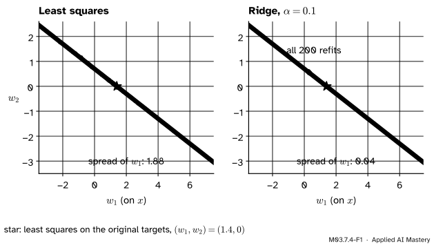
Refit the wobbly design on two hundred copies of the targets, each with fresh noise of size about \(0.1\), and plot the two duplicate weights.
M03.7.4-F1
Each dot is one refit on slightly noisy targets. Least squares sends the two duplicate weights all along one line; ridge keeps them in a tight cluster near the shared answer of the last lesson.
The streak lies along one direction, \(\vect{v}_3\), the direction in weight space in which the two copies trade off against each other: more on \(x\), less on the copy. Moving along it barely changes the predictions, because the copies are so alike. So the data hardly constrain the weights in that direction, and the noise is free to push them about. Ridge charges a price for long weight vectors (ML01.9.1), and that price is felt most exactly where the data say least.
Build it up
Step 1. The SVD sum. Lesson M03.7.2 wrote the least-squares solution as one term per singular direction:
Step 2. Follow the noise. Replace \(\vect{b}\) by \(\vect{b} + \vect{d}\), where \(\vect{d}\) is a small disturbance. The sum is linear in \(\vect{b}\), so the weights change by \(\sum_i {(\vect{u}_i \cdot \vect{d})/\sigma_i}\;\vect{v}_i\). The part of the noise along \(\vect{u}_i\) is divided by \(\sigma_i\), which multiplies it by \(1/\sigma_i\).
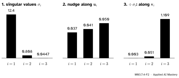
Step 3. Look at the numbers. For the wobbly design the singular values are about \(12.38\), \(0.808\) and \(0.0447\). The nudge of \(0.1\) on the second target has parts of sizes \(0.037\), \(0.041\) and \(0.050\) along \(\vect{u}_1, \vect{u}_2, \vect{u}_3\): much the same. After the division they are \(0.003\), \(0.051\) and \(1.11\).
M03.7.4-F2
A nudge of \(0.1\) on one target. It is spread evenly over the three \(\vect{u}\)-directions, but the third part is divided by \(\sigma_3 \approx 0.045\) and arrives in the weights about 22 times larger.
Step 4. Two cures. Either drop the terms with small \(\sigma_i\) altogether, or damp them. The first is truncated SVD; the second, it turns out, is ridge.
The formal statement
Let \(\mat{A}\) be \(m \times n\) with \(m \ge n\) and thin SVD \(\mat{A} = \mat{U}\mat{\Sigma}\mat{V}\T\), so \(\mat{V}\) is square and orthogonal. For \(\alpha > 0\) the ridge solution minimises \({\norm{\vect{b} - \mat{A}\vect{x}}^2} + {\alpha\norm{\vect{x}}^2}\). Its gradient is \({-2\mat{A}\T(\vect{b} - \mat{A}\vect{x})} + {2\alpha\vect{x}}\), as in ML01.9.1, and setting it to zero gives
where the inverse exists because, as the derivation below shows, the eigenvalues of \(\mat{A}\T\mat{A} + \alpha\mat{I}\) are \(\sigma_i^2 + \alpha > 0\).
The middle factor is diagonal with entries \(\sigma_i^2 + \alpha > 0\), so the inverse is \(\mat{V}(\mat{\Sigma}^2 + \alpha\mat{I})^{-1}\mat{V}\T\) (multiply the two to check). Now multiply by \(\mat{A}\T\vect{b} = \mat{V}\mat{\Sigma}\mat{U}\T\vect{b}\) and cancel \(\mat{V}\T\mat{V} = \mat{I}\):
The diagonal matrix in the middle has entries \(\sigma_i/(\sigma_i^2 + \alpha)\). Read column by column, that is the sum \(\sum_i {\sigma_i\,(\vect{u}_i \cdot \vect{b})/(\sigma_i^2 + \alpha)}\;\vect{v}_i\). Finally, for \(\sigma_i > 0\),
and for \(\sigma_i = 0\) the entry is \(0\). The limit. As \(\alpha \to 0\), each \(f_i\) with \(\sigma_i > 0\) tends to \(1\), while the terms with \(\sigma_i = 0\) stay \(0\) for every \(\alpha\). What remains is \(\sum_{\sigma_i > 0} {(\vect{u}_i \cdot \vect{b})/\sigma_i}\;\vect{v}_i = \mat{A}^+\vect{b}\). \(\blacksquare\)
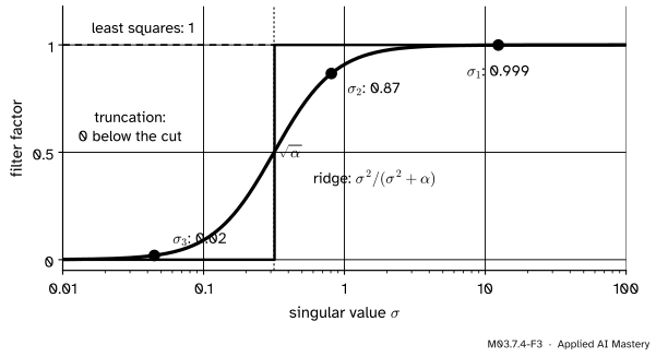
Reading the filter. A term with \(\sigma_i^2\) much larger than \(\alpha\) keeps \(f_i \approx 1\); one with \(\sigma_i^2\) much smaller is damped to \(f_i \approx \sigma_i^2/\alpha\), which cancels the dangerous \(1/\sigma_i\): the term becomes \(\sigma_i(\vect{u}_i \cdot \vect{b})/\alpha\), small. The switch happens near \(\sigma_i = \sqrt{\alpha}\), where \(f_i = \tfrac12\). Truncated SVD uses the sharp version: \(f_i = 1\) if \(\sigma_i\) is above a chosen cut and \(f_i = 0\) below it.
M03.7.4-F3
The filter factors with \(\alpha = 0.1\). Ridge fades the terms smoothly as \(\sigma\) falls below \(\sqrt{\alpha}\); truncation switches them off. On the wobbly design ridge keeps \(0.999\) of the first term, \(0.87\) of the second and \(0.02\) of the third.
Go deeper: the same price in two conventions
Lesson ML01.9.1 adds \(\lambda\norm{\vect{w}}^2\) to the mean squared error, \(\tfrac1n\norm{\vect{y} - \mat{X}\vect{w}}^2\). Multiply that loss by \(n\) and it becomes \({\norm{\vect{y} - \mat{X}\vect{w}}^2} + {n\lambda\norm{\vect{w}}^2}\), the form used here. Multiplying a loss by a positive constant does not move its minimum, so the two describe the same weights when \(\alpha = n\lambda\). scikit-learn’s Ridge uses the sum, so its alpha is our \(\alpha\).
Worked example
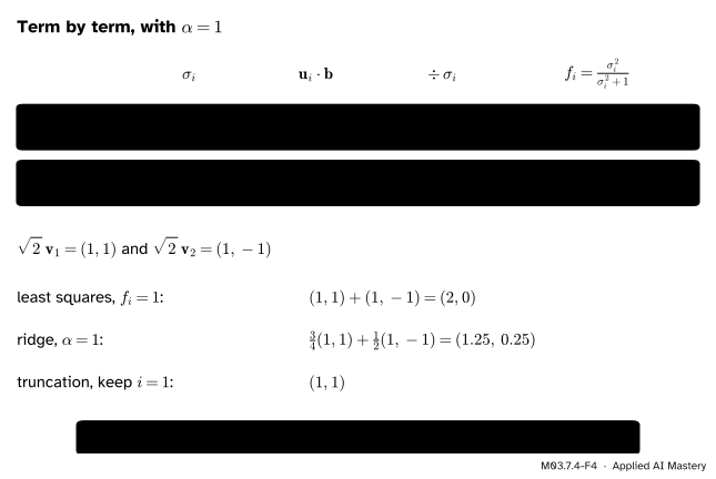
The running \(\mat{B}\) with \(\vect{b} = (3, 1, -1)\) and \(\alpha = 1\).
The pieces. From lesson M03.7.2, \(\sigma_1 = \sqrt{3}\), \(\sigma_2 = 1\), \(\vect{u}_1 = (2, 1, 1)/\sqrt{6}\), \(\vect{u}_2 = (0, 1, -1)/\sqrt{2}\), \(\vect{v}_1 = (1, 1)/\sqrt{2}\), \(\vect{v}_2 = (1, -1)/\sqrt{2}\). Then
Least squares jumps by about \(1\) in the weight on \(x\); ridge and truncation move by a few hundredths. Both stay close to the shared answer \((0.5, 0.28, 0.56)\) of the last lesson. Now scikit-learn, and the limit \(\alpha \to 0\) on the exact duplicate.
model = Ridge(alpha=0.1, fit_intercept=False).fit(A, y)print("sklearn Ridge:", np.round(model.coef_, 4), " ours:", np.round(filtered(A, y, ridge(0.1)), 4))D = np.column_stack([np.ones(4), x, 2* x])for alpha in (1.0, 1e-2, 1e-4, 1e-8):print(f"alpha = {alpha:g}:", np.round(np.linalg.solve(D.T @ D + alpha * np.eye(3), D.T @ y), 5))print("pinv:", np.round(np.linalg.pinv(D) @ y, 5))
With fit_intercept=False and the column of ones inside A, scikit-learn minimises exactly \({\norm{\vect{y} - \mat{A}\vect{w}}^2} + {\alpha\norm{\vect{w}}^2}\), and the weights agree. As \(\alpha\) shrinks on the exact duplicate, ridge walks to the pseudoinverse solution.
Frontier note: gradient descent finds the minimum-norm solution
Run gradient descent on \(\norm{\vect{b} - \mat{A}\vect{w}}^2\) from \(\vect{w}_0 = \vect{0}\). Each step adds a multiple of \(\mat{A}\T(\vect{b} - \mat{A}\vect{w}_t)\), a combination of the rows of \(\mat{A}\), so every iterate stays in the row space. With a small enough step the iterates converge to a least-squares solution that lies in the row space, and that is \(\mat{A}^+\vect{b}\) (Hastie, Montanari, Rosset and Tibshirani, Proposition 1). No penalty was written down, yet the method chose the shortest answer. In over-parameterised models, with more weights than examples, this minimum-norm interpolation fits the training data exactly; Hastie and co-authors study when it still predicts well, and recover the “double descent” of the test error seen in large networks.
w = np.zeros(3)eta =1.0/ np.linalg.eigvalsh(D.T @ D).max() # a step no larger than 1 / lambda_maxfor _ inrange(20000): w = w + eta * D.T @ (y - D @ w)print("gradient descent from zero:", np.round(w, 6))
gradient descent from zero: [0.5 0.28 0.56]
Explore
The module’s interactive is in lesson M03.7.1. Its two columns, \((1, 1, 1)\) and \((1, 2, 3)\), are far from parallel, so no singular value is small and least squares there is calm: nudge a height by \(0.1\) and \(\hat{\vect{x}}\) moves by about as much.
Pitfalls
M03.7.4-F5
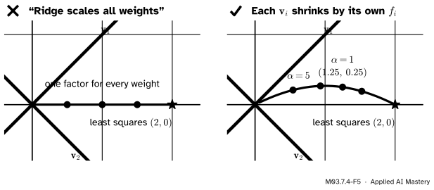
Wrong beside right, for \(\mat{B}\) and \(\vect{b} = (3, 1, -1)\). One factor for all weights would slide \((2, 0)\) straight to the origin. Ridge shrinks the weak direction \(\vect{v}_2\) faster, so its path bends towards \(\vect{v}_1\).
“Ridge multiplies every weight by the same factor.”
Only when all the singular values are equal. In general the factor depends on the direction: \(f_i = \sigma_i^2/(\sigma_i^2 + \alpha)\) along \(\vect{v}_i\). That is the point of ridge: it leaves the well-determined directions almost alone and damps the poorly determined ones hardest.
“Ridge(alpha) gives the same weights as my formula.”
Only with fit_intercept=False and the column of ones in the matrix, as above. With the default fit_intercept=True, scikit-learn fits the intercept separately and does not penalise it, so \((\mat{A}\T\mat{A} + \alpha\mat{I})^{-1}\mat{A}\T\vect{b}\), which does penalise the weight on the column of ones, gives different numbers.
“Dropping the smallest singular value drops the useless feature.”
It drops a direction, \(\vect{v}_3\), and here \(\vect{v}_3\) is close to \(\pm(0, 2, -1)/\sqrt{5}\): a mixture of both copies, the difference between them. Truncated SVD keeps both features and gives up only on telling them apart.
“\(\alpha = 0\) is best, because it adds no bias.”
It adds no bias and the most noise, as the left of the anchor figure shows. Too large an \(\alpha\) damps the strong directions too. The trade-off is chosen on held-out data, by cross-validation (ML01.9.3).
Check yourself
Recall
1. Why does a small singular value make least squares sensitive to noise?
Show answer
The part of the noise along \(\vect{u}_i\) enters the weights as \({(\vect{u}_i \cdot \vect{d})/\sigma_i}\), multiplied by \(1/\sigma_i\).
2. What is the ridge filter factor of the term with singular value \(\sigma_i\)?
Show answer
\(f_i = \sigma_i^2/(\sigma_i^2 + \alpha)\).
3. Where does the ridge filter equal one half?
Show answer
At \(\sigma_i = \sqrt{\alpha}\).
4. What does the ridge solution tend to as \(\alpha \to 0\)?
Show answer
The minimum-norm least-squares solution \(\mat{A}^+\vect{b}\).
5. What are the filter factors of truncated SVD?
Show answer
1 for every \(\sigma_i\) above the cut, 0 for every one below it.
Exercises
1.★ With \(\alpha = 1\), find the ridge filter factors for singular values \(3\), \(1\) and \(0.1\).
Show solution
\(f = 9/10 = 0.9\), then \(1/2 = 0.5\), then \(0.01/1.01 \approx 0.0099\). The smallest term keeps less than one per cent of itself, which also cancels the factor \(1/0.1 = 10\) it would otherwise bring.
2.★★ For \(\mat{B}\) and \(\vect{b} = (3, 0, 0)\) find the least-squares, ridge (\(\alpha = 1\)) and truncated (keep \(i = 1\)) weights, and check ridge by \((\mat{B}\T\mat{B} + \mat{I})^{-1}\mat{B}\T\vect{b}\).
Show solution
From lesson M03.7.2, \(\vect{u}_1 \cdot \vect{b} = \sqrt{6}\) and \(\vect{u}_2 \cdot \vect{b} = 0\). Least squares: \(\sqrt{2}\,\vect{v}_1 = (1, 1)\). Truncation keeps the same single term: \((1, 1)\). Ridge: \(\tfrac34(1, 1) = (0.75, 0.75)\). Check: \(\mat{B}\T\vect{b} = (3, 3)\) and
In each term the numerator does not depend on \(\alpha\), and the denominator \((\sigma_i^2 + \alpha)^2\) grows with \(\alpha\). So each term, and the sum, can only shrink or stay the same. As \(\alpha \to \infty\) every term tends to \(0\) and the weights to \(\vect{0}\); as \(\alpha \to 0\) the length rises to \(\norm{\mat{A}^+\vect{b}}\).
Summary card
Small singular values amplify noise; ridge and truncation filter them.
M03.7.4-F1
Noise along \(\vect{v}_3\), tamed.
Least squares.\(\hat{\vect{x}} = \sum_i {(\vect{u}_i \cdot \vect{b})/\sigma_i}\;\vect{v}_i\): noise times \(1/\sigma_i\).
Limit.\(\vect{x}_\alpha \to \mat{A}^+\vect{b}\) as \(\alpha \to 0\).
Sources and next steps
Sources. Each was opened and checked against this lesson on 15 November 2026.
Julianne Chung and Silvia Gazzola, Computational methods for large-scale inverse problems: a survey on hybrid projection methods, published in 2021. Equation (2.1), at the start of Section 2, is the standard-form Tikhonov problem \({\norm{\vect{b} - \mat{A}\vect{x}}^2} + {\lambda\norm{\vect{x}}^2}\), and equation (2.2), in subsection 2.1, gives its solution as a sum over the SVD with the Tikhonov filter factors \(\sigma_i^2/(\sigma_i^2 + \lambda)\); the same subsection gives the truncated SVD as the filter with factors 1 for \(i \le k\) and 0 otherwise. Their \(\lambda\) is our \(\alpha\).
scikit-learn, sklearn.linear_model.Ridge. The objective \({\norm{\vect{y} - \mat{X}\vect{w}}^2} + {\alpha\norm{\vect{w}}^2}\), the meaning of fit_intercept, and the remark that alpha = 0 is not advised.
Trevor Hastie, Andrea Montanari, Saharon Rosset and Ryan Tibshirani, Surprises in high-dimensional ridgeless least squares interpolation (2019). Proposition 1: gradient descent from zero with a step of at most \(1/\lambda_{\max}\) converges to the minimum-norm least-squares solution; and the minimum-norm estimator as the limit of ridge as the penalty tends to zero.
Next. This completes the module. M03.8 Matrix norms and conditioning turns “a small singular value is dangerous” into a number, the condition number \(\kappa\), and proves the \(\kappa(\mat{A}\T\mat{A}) = \kappa(\mat{A})^2\) that lesson M03.7.2 only measured.