Multiply the SVD out and any matrix becomes a sum of rank-one layers, each a column times a row, largest first. Derive it, rebuild two matrices layer by layer, read off the largest stretch and the sum of squared entries, and compare the SVD of a symmetric matrix with its eigenvalues.
M03.5.4L2 Intermediate25 minIn review (what this means)
The maths and code on this page are checked by automated tests on every change, but an independent reader has not signed it off yet. Spot a mistake or a confusing step? Tell us.
Derive A = sigma_1 u_1 v_1-transpose + … + sigma_r u_r v_r-transpose from the product U Sigma V-transpose, and explain why each layer has rank one.
Rebuild a small matrix layer by layer and say how big the error is after each layer.
Show that the largest stretch of A is sigma_1 and that the sum of the squared entries of A equals the sum of the squared singular values.
Relate the SVD of a symmetric matrix to its eigendecomposition, for positive definite and for indefinite matrices.
The question
A photograph is a matrix of brightness values, and so is the weight matrix of a neural network layer. Can such a matrix be written as a sum of very simple pieces, ranked from most to least important, so that keeping only the first few pieces keeps most of the matrix? And how would we measure what the rest are worth?
From the last lesson
1. How do you read the rank of a matrix off its SVD?
Show answer
It is the number of positive singular values; in floating point, the number above a tolerance.
2. Which columns of \(\mat{U}\) span the column space, and which span the left null space?
Show answer
\(\vect{u}_1, \dots, \vect{u}_r\) span the column space; \(\vect{u}_{r+1}, \dots, \vect{u}_m\) span the left null space.
Intuition
The simplest non-zero matrix is a column times a row, \(\vect{u}\vect{v}\T\): a multiplication table. Every row of it is a multiple of the same row \(\vect{v}\T\), so it has rank one. Call such a matrix a rank-one layer.
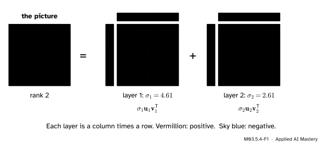
The SVD says that every matrix is a stack of such layers, one for each singular value, with the biggest first. Look at the picture of a cross below. It is the sum of exactly two layers. The first layer alone already shows a blurred cross; the second adds the corrections, positive along the arms and negative at the centre and in the corners.
M03.5.4-F1
A picture of a cross, as a matrix, is the sum of two rank-one layers. Each layer is a column (left strip) times a row (top strip). Lesson M03.6.2 does the same with a real photograph and many layers.
Build it up
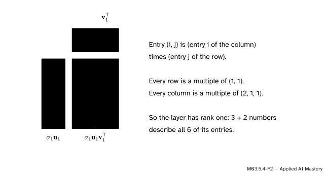
Step 1. A column times a row. For a column \(\vect{u}\) with \(m\) entries and a row \(\vect{v}\T\) with \(n\) entries, the outer product\(\vect{u}\vect{v}\T\) is the \(m\) by \(n\) matrix whose entry \((i, j)\) is \(u_iv_j\). Row \(i\) is \(u_i\vect{v}\T\) and column \(j\) is \(v_j\vect{u}\). So every row is a multiple of one row, every column is a multiple of one column, and \(m + n\) numbers describe all \(mn\) entries.
M03.5.4-F2
The first layer of the running rectangular matrix \(\mat{B}\) as a multiplication table.
Step 2. What a layer does to a vector. Multiply a layer by an input \(\vect{x}\) and regroup:
The layer measures how much of \(\vect{x}\) points along \(\vect{v}\), scales that by \(\sigma\), and sends the result out along \(\vect{u}\). That is one turn, one stretch and one turn, for a single direction.
Step 3. A product as a sum of columns times rows. Let \(\mat{X}\) have columns \(\vect{c}_1, \dots, \vect{c}_k\) and let \(\mat{Y}\) have rows \(\vect{r}_1\T, \dots, \vect{r}_k\T\). Entry \((i, j)\) of \(\mat{X}\mat{Y}\) is \({x_{i1}y_{1j} + \dots + x_{ik}y_{kj}}\), and the term \(x_{il}y_{lj}\) is exactly entry \((i, j)\) of the outer product \(\vect{c}_l\vect{r}_l\T\). Adding over \(l\):
Apply Step 3 to the thin SVD, with \(\mat{X} = \mat{U}\mat{\Sigma}\) and \(\mat{Y} = \mat{V}\T\). Column \(i\) of \(\mat{U}\mat{\Sigma}\) is \(\sigma_i\vect{u}_i\), and row \(i\) of \(\mat{V}\T\) is \(\vect{v}_i\T\). Terms with \(\sigma_i = 0\) vanish. So:
with \(r\) the rank and \({\sigma_1 \ge \dots \ge \sigma_r > 0}\). Applied to a vector, \(\mat{A}\vect{x} = \sum_i \sigma_i\,{(\vect{v}_i \cdot \vect{x})}\,\vect{u}_i\).
Each layer has rank one, and the layers are as separate as they can be: their \(\vect{u}\)’s are perpendicular and so are their \(\vect{v}\)’s. Two consequences preview the matrix norms of M03.8.1.
The largest stretch is \(\sigma_1\). For a unit vector \(\vect{x}\), \(\norm{\mat{A}\vect{x}}^2 = \vect{x}\T\mat{A}\T\mat{A}\vect{x}\). That is the Rayleigh quotient of the symmetric matrix \(\mat{A}\T\mat{A}\), which lies between its smallest and largest eigenvalues (M03.3.4). The largest eigenvalue is \(\sigma_1^2\), reached at \(\vect{v}_1\). So
which is the long half-axis of the ellipse of lesson M03.5.1.
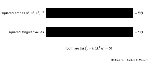
The sum of squared entries is the sum of the \(\sigma_i^2\). The diagonal entry \(j\) of \(\mat{A}\T\mat{A}\) is (column \(j\)) \(\cdot\) (column \(j\)), the sum of the squares of column \(j\). So the trace adds up every squared entry of \(\mat{A}\). The trace is also the sum of the eigenvalues (M03.1.3), which are the \(\sigma_i^2\):
This total is the square of the Frobenius norm\(\norm{\mat{A}}_F\). Since the layers come in decreasing order, the first few carry the largest share of it.
M03.5.4-F4
For \(\mat{A} = \begin{bmatrix} 3 & 0 \\ 4 & 5 \end{bmatrix}\) the squared entries and the squared singular values both add up to \(50\). The first layer carries \(45\) of the \(50\).
Symmetric matrices. The spectral theorem writes a symmetric matrix as a sum of layers too, \(\mat{S} = {\lambda_1\vect{q}_1\vect{q}_1\T + \dots + \lambda_n\vect{q}_n\vect{q}_n\T}\) (M03.3.3).
If every \(\lambda_i \ge 0\), this already is an SVD: \(\vect{u}_i = \vect{v}_i = \vect{q}_i\) and \(\sigma_i = \lambda_i\), listed largest first.
If some \(\lambda_i < 0\), write \({\lambda_i\vect{q}_i\vect{q}_i\T} = {\abs{\lambda_i}(-\vect{q}_i)\vect{q}_i\T}\). Then \(\sigma_i = \abs{\lambda_i}\), \(\vect{v}_i = \vect{q}_i\) and \(\vect{u}_i = -\vect{q}_i\): the sign moves into \(\mat{U}\). The singular values are the absolute values of the eigenvalues, re-sorted.
For a matrix that is not symmetric there is no such link, as lesson M03.5.1 showed.
From lessons 1 and 2: \(\sigma_1 = 3\sqrt{5}\), \(\vect{u}_1 = (1, 3)/\sqrt{10}\), \(\vect{v}_1 = (1, 1)/\sqrt{2}\), and \(\sigma_2 = \sqrt{5}\), \(\vect{u}_2 = (-3, 1)/\sqrt{10}\), \(\vect{v}_2 = (-1, 1)/\sqrt{2}\). In both layers the numbers in front combine as \(\sqrt{5}/{(\sqrt{10}\sqrt{2})} = \sqrt{5}/\sqrt{20} = 1/2\).
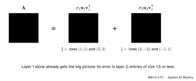
Layer 1. The outer product of \((1, 3)\) and \((1, 1)\) has rows \((1, 1)\) and \((3, 3)\); the factor in front is \({3 \cdot \tfrac12}\):
The error after one layer is layer 2. Its squared entries add to \({2.25 + 2.25 + 0.25 + 0.25} = 5 = \sigma_2^2\), a tenth of the total \(50\). Lesson M03.6.1 proves that no other rank-one matrix comes closer to \(\mat{A}\).
M03.5.4-F3
The running SVD matrix rebuilt from its two layers.
Code
From scratch: the layers from the factors, the running totals, and the two facts of the formal statement, for \(\mat{A}\) and for the rectangular \(\mat{B}\).
import numpy as npdef layers(M):"""The rank-one layers sigma_i u_i v_i^T of a matrix, largest first.""" U, s, Vh = np.linalg.svd(M, full_matrices=False)return [s[i] * np.outer(U[:, i], Vh[i]) for i inrange(len(s)) if s[i] >1e-12* s[0]]A = np.array([[3.0, 0.0], [4.0, 5.0]])B = np.array([[1.0, 1.0], [1.0, 0.0], [0.0, 1.0]])for name, M in (("A", A), ("B", B)): total = np.zeros_like(M)for k, L inenumerate(layers(M), start=1): total = total + Lprint(f"{name}, layer {k}:", (np.round(L, 6) +0.0).tolist()," rank", np.linalg.matrix_rank(L)," squared error left:", round(np.sum((M - total) **2), 6))
The signs inside each layer cancel (\(\vect{u}_i\) and \(\vect{v}_i\) flip together), so the layers are the same whichever signs the library chose. Now the largest stretch, by trying many random directions, and the sum of squares:
rng = np.random.default_rng(1)angles = rng.uniform(0, 2* np.pi, 100_000)X = np.vstack([np.cos(angles), np.sin(angles)]) # 100,000 unit vectors as columnsstretch = np.linalg.norm(A @ X, axis=0)s = np.linalg.svd(A, compute_uv=False)print("largest stretch found:", round(stretch.max(), 6), " sigma_1:", round(s[0], 6))print("sum of squared entries:", np.sum(A **2), " sum of sigma^2:", round(np.sum(s **2), 9))
largest stretch found: 6.708204   sigma_1: 6.708204
sum of squared entries: 50.0   sum of sigma^2: 50.0
Finally, symmetric matrices: the running bowl \(\mat{S}\) and the running saddle.
For the saddle, \(\vect{u}_2 \cdot \vect{v}_2 = -1\): the left and right singular vectors of the second layer point in opposite directions, which is where the eigenvalue’s minus sign went.
Frontier note: low-rank updates in fine-tuning
Fine-tuning adapts a pretrained network to a new task by changing its weight matrices. A weight matrix \(\mat{W}_0\) of size \({d \times k}\) has \(dk\) numbers. LoRA (Hu and colleagues, 2021) freezes \(\mat{W}_0\) and learns only a change that is a product of two thin matrices, of sizes \({d \times r}\) and \({r \times k}\) with \(r\) much smaller than \(d\) and \(k\): by Step 3, a sum of \(r\) rank-one layers. The layer then computes \(\mat{W}_0\vect{x}\) plus that low-rank change applied to \(\vect{x}\). With \(d = k = 4096\) and \(r = 8\), the change has \({8 \cdot (4096 + 4096)} = 65{,}536\) numbers instead of \(4096^2 = 16{,}777{,}216\): 256 times fewer. The bet behind it is that the change a new task needs has most of its weight in a few layers, which is what a fast-falling list of singular values means. Module A02.5 builds this in full.
Explore
The module’s interactive, Rotate, stretch, rotate, is in lesson M03.5.1. Choose the symmetric preset, then the saddle: in the first the singular values equal the eigenvalues, in the second one eigenvalue is negative and the read-out reports its absolute value as a singular value.
Pitfalls
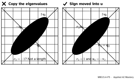
M03.5.4-F5
Wrong beside right. The saddle flips \(\vect{q}_2\), so its eigenvalue there is \(-1\). A singular value is a length, so it is \(1\), and the flip is carried by \(\vect{u}_2 = -\vect{v}_2\).
“For a symmetric matrix the singular values are the eigenvalues.”
Only when no eigenvalue is negative. The saddle has eigenvalues \(3\) and \(-1\), but singular values \(3\) and \(1\). The ellipse’s half-axes are lengths; the minus sign says that the second axis is turned round, and the SVD records that in \(\mat{U}\).
“The first layer is the first row (or the biggest entries) of the matrix.”
A layer is a column times a row, so it is zero only in the rows where \(\vect{u}_i\) has a zero and the columns where \(\vect{v}_i\) has a zero. Usually it spreads over every entry: layer 1 of \(\mat{A}\) changes all four entries, and so does layer 2. So truncating the sum usually changes many entries a little rather than a few entries a lot; that is why a compressed photograph gets blurred rather than holed (M03.6.2).
“\(\vect{u}\vect{v}\T\) and \(\vect{u}\T\vect{v}\) are the same thing.”
\(\vect{u}\T\vect{v}\), a row times a column, is a single number, the dot product. \(\vect{u}\vect{v}\T\), a column times a row, is a whole matrix. In NumPy, u @ v gives the number and np.outer(u, v) gives the matrix.
Check yourself
Recall
1. Write a matrix of rank \(r\) as a sum of layers using its SVD.
2. Why does the outer product \(\vect{u}\vect{v}\T\) of two non-zero vectors have rank one?
Show answer
Row \(i\) is \(u_i\vect{v}\T\), so every row is a multiple of one row; the row space is a line.
3. What is the largest value of \(\norm{\mat{A}\vect{x}}\) over unit vectors, and where is it reached?
Show answer
\(\sigma_1\), at \(\vect{x} = \vect{v}_1\).
4. What does the sum of the squares of the entries of \(\mat{A}\) equal?
Show answer
\(\operatorname{tr}(\mat{A}\T\mat{A}) = \sigma_1^2 + \dots + \sigma_r^2\), the squared Frobenius norm. For the running \(\mat{A}\), \(50 = 45 + 5\).
5. How do the singular values of a symmetric matrix relate to its eigenvalues?
Show answer
They are the absolute values of the eigenvalues, sorted largest first. For a negative eigenvalue the sign moves into \(\vect{u}_i = -\vect{q}_i\).
Exercises
1.★ Show that \(\mat{R} = \begin{bmatrix} 2 & 2 \\ 1 & 1 \end{bmatrix}\) is a single layer \(\sigma_1\vect{u}_1\vect{v}_1\T\), and check the sum-of-squares rule on it.
Show solution
From lesson M03.5.3, \(\sigma_1 = \sqrt{10}\), \(\vect{u}_1 = (2, 1)/\sqrt{5}\) and \(\vect{v}_1 = (1, 1)/\sqrt{2}\). The factor in front is \({\sqrt{10}/(\sqrt{5}\sqrt{2})} = 1\), and the outer product of \((2, 1)\) and \((1, 1)\) has rows \((2, 2)\) and \((1, 1)\), which is \(\mat{R}\). The squared entries add to \({4 + 4 + 1 + 1} = 10 = \sigma_1^2\).
2.★★ Write \(\mat{S} = \begin{bmatrix} 2 & 1 \\ 1 & 2 \end{bmatrix}\) and the saddle \(\begin{bmatrix} 1 & 2 \\ 2 & 1 \end{bmatrix}\) each as a sum of two SVD layers, and check by adding.
Show solution
With \(\vect{q}_1 = (1, 1)/\sqrt{2}\) and \(\vect{q}_2 = (1, -1)/\sqrt{2}\), the outer products are \(\vect{q}_1\vect{q}_1\T = \tfrac12\) (rows \((1, 1)\), \((1, 1)\)) and \(\vect{q}_2\vect{q}_2\T = \tfrac12\) (rows \((1, -1)\), \((-1, 1)\)). For \(\mat{S}\), \(\sigma = 3, 1\) and \(3\vect{q}_1\vect{q}_1\T + 1\vect{q}_2\vect{q}_2\T\) has rows \({(1.5 + 0.5,\; 1.5 - 0.5)} = (2, 1)\) and \((1, 2)\). For the saddle, \(\sigma = 3, 1\) with \(\vect{u}_2 = -\vect{q}_2\): \({3\vect{q}_1\vect{q}_1\T + 1(-\vect{q}_2)\vect{q}_2\T}\) has rows \({(1.5 - 0.5,\; 1.5 + 0.5)} = (1, 2)\) and \((2, 1)\).
3.★★★ Prove that the error left after the first layer satisfies \(\norm{\mat{A} - \sigma_1\vect{u}_1\vect{v}_1\T}_F^2 = \sigma_2^2 + \dots + \sigma_r^2\).
Show solution
The error is \(\mat{E} = {\sigma_2\vect{u}_2\vect{v}_2\T + \dots + \sigma_r\vect{u}_r\vect{v}_r\T}\). Its squared Frobenius norm is \(\operatorname{tr}(\mat{E}\T\mat{E})\). Multiply out, using \((\vect{u}_i\vect{v}_i\T)\T = \vect{v}_i\vect{u}_i\T\):
The \(\vect{u}\)’s are orthonormal, so only the terms with \(i = j\) survive, each with \(\vect{u}_i \cdot \vect{u}_i = 1\): \(\mat{E}\T\mat{E} = {\sum_{i \ge 2} \sigma_i^2\vect{v}_i\vect{v}_i\T}\). The trace of \(\vect{v}_i\vect{v}_i\T\) is \({v_{i1}^2 + \dots + v_{in}^2} = 1\), and the trace of a sum is the sum of the traces, so the total is \({\sigma_2^2 + \dots + \sigma_r^2}\). For the running \(\mat{A}\) that is \(5\), as the worked example found.
Summary card
Every matrix is a sum of rank-one layers \(\sigma_i\vect{u}_i\vect{v}_i\T\), largest first.
M03.5.4-F1
Two layers make the cross.
Layers.\(\mat{A} = {\sum_{i=1}^r \sigma_i\vect{u}_i\vect{v}_i\T}\); each \(\vect{u}\vect{v}\T\) has rank one.
Symmetric.\(\sigma_i = \abs{\lambda_i}\); a negative sign moves into \(\vect{u}_i\).
Sources and next steps
Sources. Each was opened and checked against this lesson on 15 November 2026.
David Austin, Understanding Linear Algebra, section “Using singular value decompositions”: \(\mat{A}\) written as a sum of outer products \(\sigma_i\vect{u}_i\vect{v}_i\T\), each of rank one, and the rank \(k\) approximations made from the first \(k\) of them.
Marc Peter Deisenroth, A. Aldo Faisal and Cheng Soon Ong, Mathematics for Machine Learning, Section 4.6, equation (4.91): a matrix of rank \(r\) as the sum of the rank-1 matrices \(\sigma_i\vect{u}_i\vect{v}_i\T\).
Sheldon Axler, Linear Algebra Done Right, 4th edition: formula 7.71 in the SVD 7.70, \(Tv = s_1\langle v, e_1\rangle f_1 + \dots\) (the action of the layers), and 7.82 to 7.85 in Section 7F: \(\norm{Tv} \le s_1\norm{v}\), with equality at \(e_1\).
Edward J. Hu, Yelong Shen, Phillip Wallis and others, LoRA: Low-Rank Adaptation of Large Language Models, 2021, Section 4.1 and equation (3): the pretrained \(W_0\) is frozen and the update is a product of a \({d \times r}\) and an \({r \times k}\) matrix, with \(h = W_0x + BAx\).
Next. M03.6.1, The best rank-k approximation, in the course outline, keeps only the first \(k\) layers and proves that nothing of rank \(k\) does better; M03.8.1 turns \(\sigma_1\) and the sum of squares into the matrix norms \(\norm{\mat{A}}_2\) and \(\norm{\mat{A}}_F\).