The right singular vectors of any matrix are the eigenvectors of the symmetric matrix A-transpose A, and the singular values are the square roots of its eigenvalues. Use this to compute an SVD by hand, prove that every matrix has one, and see why a library never forms A-transpose A.
M03.5.2L2 Intermediate25 minIn review (what this means)
The maths and code on this page are checked by automated tests on every change, but an independent reader has not signed it off yet. Spot a mistake or a confusing step? Tell us.
Derive A-transpose A = V Sigma-squared V-transpose from A = U Sigma V-transpose, and explain why A-transpose A is symmetric and positive semidefinite.
Compute the SVD of a 2 by 2 matrix by hand: eigenvalues and eigenvectors of A-transpose A, then sigma_i = sqrt(lambda_i) and u_i = A v_i / sigma_i.
Prove that the vectors u_i built this way are orthonormal, and so that every matrix has a singular value decomposition.
Build an SVD from numpy.linalg.eigh, compare it with numpy.linalg.svd, and explain the differences in sign and order.
The question
The last lesson found the singular vectors of a 2 by 2 matrix by turning a pair of arrows until their images met at a right angle. A matrix of a thousand columns cannot be searched like that. Is there a direct way to find the singular vectors, and can we be sure that every matrix, of any size, has them?
From the last lesson
1. State the equation that links \(\vect{v}_i\), \(\sigma_i\) and \(\vect{u}_i\).
Show answer
\(\mat{A}\vect{v}_i = \sigma_i\vect{u}_i\): the unit input \(\vect{v}_i\) lands on the axis \(\vect{u}_i\) of the ellipse, at distance \(\sigma_i\) from the centre.
2. What are the singular values of \(\begin{bmatrix} 3 & 0 \\ 4 & 5 \end{bmatrix}\), and how does their product compare with the determinant?
Show answer
\(\sigma_1 = 3\sqrt{5} \approx 6.708\) and \(\sigma_2 = \sqrt{5} \approx 2.236\). Their product is \(15 = \det\mat{A}\).
Intuition
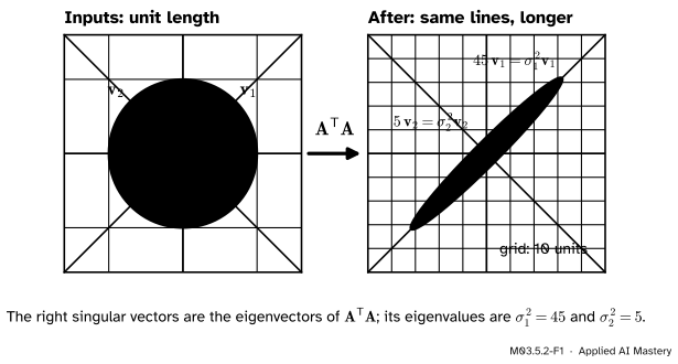
Follow a right singular vector there and back. The matrix \(\mat{A}\) sends \(\vect{v}_1\) to \(\sigma_1\vect{u}_1\). The transpose \(\mat{A}\T\) runs the other way, from outputs back to inputs, and it sends \(\vect{u}_1\) back to \(\sigma_1\vect{v}_1\) (we prove this below). So the round trip \(\mat{A}\T\mat{A}\) brings \(\vect{v}_1\) home to its own line, stretched by \(\sigma_1^2\).
That is an eigenvector statement. The right singular vectors of \(\mat{A}\) are the eigenvectors of \(\mat{A}\T\mat{A}\), and the squared singular values are its eigenvalues. Since \(\mat{A}\T\mat{A}\) is symmetric, the spectral theorem of M03.3 hands us its eigenvectors, perpendicular and ready made.
M03.5.2-F1
The round trip \(\mat{A}\T\mat{A}\) for \(\mat{A} = \begin{bmatrix} 3 & 0 \\ 4 & 5 \end{bmatrix}\). It keeps \(\vect{v}_1\) and \(\vect{v}_2\) on their own lines and stretches them by \(45\) and \(5\).
Build it up
Step 1. Assume an SVD and multiply. Suppose \(\mat{A} = \mat{U}\mat{\Sigma}\mat{V}\T\). The transpose of a product is the product of the transposes in reverse order, so \(\mat{A}\T = \mat{V}\mat{\Sigma}\T\mat{U}\T\). For a square matrix \(\mat{\Sigma}\) is diagonal, so \(\mat{\Sigma}\T = \mat{\Sigma}\). Then
because \(\mat{U}\T\mat{U} = \mat{I}\). This is exactly the form \({\mat{Q}\mat{\Lambda}\mat{Q}\T}\) of the spectral theorem (M03.3.2): orthonormal eigenvectors \(\vect{v}_i\), eigenvalues \(\sigma_i^2\). Multiplying \(\mat{A}\T = \mat{V}\mat{\Sigma}\mat{U}\T\) by \(\mat{U}\) also proves the claim of the intuition, column by column: \(\mat{A}\T\vect{u}_i = \sigma_i\vect{v}_i\).
Step 2. Turn it round. Step 1 assumed the SVD. To find it, start from \(\mat{A}\T\mat{A}\), which we can always form, and check that it has what the spectral theorem needs.
It is symmetric: \({(\mat{A}\T\mat{A})\T} = \mat{A}\T(\mat{A}\T)\T = \mat{A}\T\mat{A}\).
It is positive semidefinite (M03.4.2): for every \(\vect{x}\),
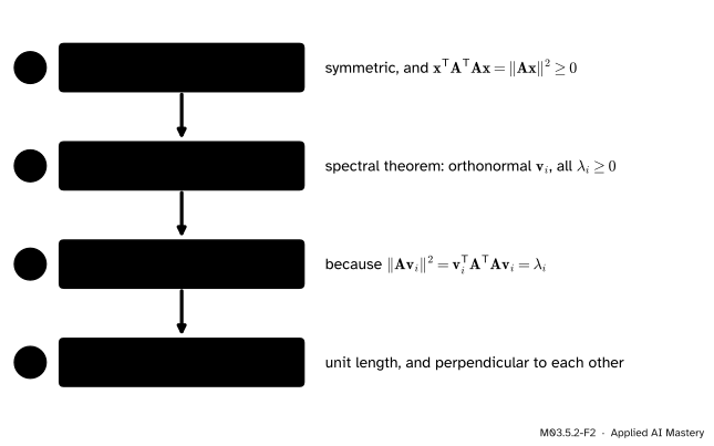
so the stretch is \(\sigma_i = \sqrt{\lambda_i}\), and \(\vect{u}_i = \mat{A}\vect{v}_i/\sigma_i\) has length one. The four steps of the recipe are below.
M03.5.2-F2
The recipe for an SVD, with the reason each step works.
The formal statement
NoteTheorem: every matrix has a singular value decomposition
Let \(\mat{A}\) be any real \(m\) by \(n\) matrix. Let \(\vect{v}_1, \dots, \vect{v}_n\) be orthonormal eigenvectors of \(\mat{A}\T\mat{A}\) with eigenvalues \({\lambda_1 \ge \dots \ge \lambda_n \ge 0}\), and put \(\sigma_i = \sqrt{\lambda_i}\). Then for each \(\sigma_i > 0\) the vectors \(\vect{u}_i = \mat{A}\vect{v}_i/\sigma_i\) are orthonormal, \(\mat{A}\vect{v}_i = \sigma_i\vect{u}_i\), and \(\mat{A}\vect{v}_i = \vect{0}\) whenever \(\sigma_i = 0\).
Proof. The eigenvectors and the non-negative eigenvalues exist by Step 2. Take two indices \(i\) and \(j\) with \(\sigma_i, \sigma_j > 0\). Move \(\mat{A}\) across the dot product as a transpose:
If \(i \ne j\), then \({\vect{v}_i \cdot \vect{v}_j} = 0\) and the \(\vect{u}\)’s are perpendicular. If \(i = j\), the fraction is \(\lambda_i / \sigma_i^2 = 1\), so each has length one. Finally, if \(\sigma_i = 0\), Step 3 gives \(\norm{\mat{A}\vect{v}_i}^2 = 0\), so \(\mat{A}\vect{v}_i = \vect{0}\). \(\blacksquare\)
For a square matrix with no zero singular value this is the whole SVD: the \(\vect{u}_i\) fill the columns of \(\mat{U}\), and \(\mat{A}\mat{V} = \mat{U}\mat{\Sigma}\) column by column, so \(\mat{A} = \mat{U}\mat{\Sigma}\mat{V}\T\) as in lesson M03.5.1. The proof also answers the question of lesson 1 for every size at once: the perpendicular inputs that stay perpendicular are the eigenvectors of \(\mat{A}\T\mat{A}\), because the dot product of two images is \(\vect{v}_i\T\mat{A}\T\mat{A}\vect{v}_j\).
Go deeper: the general case: zero singular values and rectangular matrices
When some \(\sigma_i\) are zero, or \(m \ne n\), there are fewer \(\vect{u}_i\) than the \(m\) columns of \(\mat{U}\) need. Say \(r\) singular values are positive. The vectors \(\vect{u}_1, \dots, \vect{u}_r\) are orthonormal in \(\R^m\), so Gram-Schmidt (M02.10.3), applied to them followed by the standard basis, extends them to an orthonormal basis \(\vect{u}_1, \dots, \vect{u}_m\) of \(\R^m\). Let \(\mat{U}\) hold all \(m\) of them, \(\mat{V}\) all \(n\) of the \(\vect{v}_i\), and let \(\mat{\Sigma}\) be the \(m\) by \(n\) matrix with \(\sigma_1, \dots, \sigma_r\) down its diagonal and zeros elsewhere. Check \(\mat{A}\mat{V} = \mat{U}\mat{\Sigma}\) column by column. For \(i \le r\), column \(i\) is \(\mat{A}\vect{v}_i = \sigma_i\vect{u}_i\) on both sides. For \(i > r\), the left side is \(\mat{A}\vect{v}_i = \vect{0}\), and column \(i\) of \(\mat{\Sigma}\) is zero, so the right side is \(\vect{0}\) too. Multiplying on the right by \(\mat{V}\T\) gives \(\mat{A} = \mat{U}\mat{\Sigma}\mat{V}\T\). The extra \(\vect{u}\)’s are never used by \(\mat{A}\); lesson M03.5.3 shows they span the left null space. Axler proves the same theorem for linear maps between any two inner product spaces (results 7.70 and 7.80), by this very route.
Worked example
Find the SVD of \(\mat{A} = \begin{bmatrix} 3 & 0 \\ 4 & 5 \end{bmatrix}\) through \(\mat{A}\T\mat{A}\).
Form \(\mat{A}\T\mat{A}\). Its entries are dot products of the columns \((3, 4)\) and \((0, 5)\): \(9 + 16 = 25\), \(0 + 20 = 20\) and \(0 + 25 = 25\).
because \(45 + 5 = 50\) and \({45 \cdot 5} = 225\). So \(\lambda_1 = 45\) and \(\lambda_2 = 5\).
Eigenvectors. For \(\lambda_1 = 45\), the matrix \(\mat{A}\T\mat{A} - 45\mat{I}\) has rows \((-20, 20)\) and \((20, -20)\), so \(x = y\) and \(\vect{v}_1 = (1, 1)/\sqrt{2}\). For \(\lambda_2 = 5\), the rows are \((20, 20)\) twice, so \(y = -x\) and \(\vect{v}_2 = (-1, 1)/\sqrt{2}\).
Singular values and left vectors.\(\sigma_1 = \sqrt{45} = 3\sqrt{5} \approx 6.708\) and \(\sigma_2 = \sqrt{5} \approx 2.236\). Dividing the images by them, as in lesson 1:
No search was needed, and the answer matches lesson M03.5.1.
M03.5.2-F3
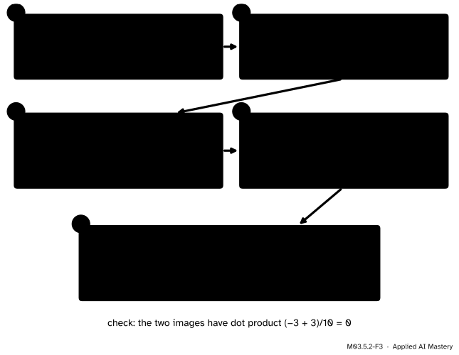
The worked example as a trace: one symmetric matrix, its eigenvalues, its eigenvectors, then square roots and one division each.
Code
From scratch: the recipe in five lines on top of numpy.linalg.eigh, which returns the eigenvalues of a symmetric matrix in ascending order, so they must be reversed.
import numpy as npdef svd_via_gram(A):"""SVD of a matrix with independent columns, through the eigenvectors of A^T A.""" lam, Q = np.linalg.eigh(A.T @ A) # ascending eigenvalues, orthonormal columns order = np.argsort(lam)[::-1] # largest first lam, V = lam[order], Q[:, order] s = np.sqrt(np.clip(lam, 0, None)) # clip a tiny negative rounding error to zero U = (A @ V) / s # column i is A v_i / sigma_ireturn U, s, VA = np.array([[3.0, 0.0], [4.0, 5.0]])U, s, V = svd_via_gram(A)print("A^T A =\n", A.T @ A)print("sigma:", s, " sigma squared:", np.round(s **2, 10))print("U^T U =\n", np.round(U.T @ U, 12))print("U Sigma V^T =\n", np.round(U @ np.diag(s) @ V.T, 12))
A^T A =
 [[25. 20.]
 [20. 25.]]
sigma: [6.70820393 2.23606798]   sigma squared: [45.  5.]
U^T U =
 [[1. 0.]
 [0. 1.]]
U Sigma V^T =
 [[3. 0.]
 [4. 5.]]
The same code works for a tall matrix with independent columns, where \(\mat{U}\) comes out with orthonormal columns but is not square (lesson M03.5.3). Now the library, which returns \(\mat{V}\T\) as Vh and the singular values in descending order:
from scratch: [3.150902 1.70933  0.334855]
numpy:        [3.150902 1.70933  0.334855]
column-by-column agreement of v (up to sign): [1. 1. 1.]
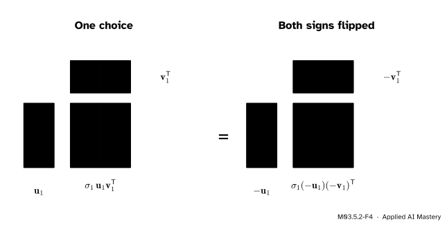
The singular values agree to every printed digit. The vectors agree up to sign: each column of \(\mat{V}\) may be flipped, as long as the matching column of \(\mat{U}\) flips with it, because the product \(\sigma_i\vect{u}_i\vect{v}_i\T\) does not change. For the running \(\mat{A}\), NumPy may well return \(-\vect{v}_1\) and \(-\vect{u}_1\). Which sign comes out depends on the LAPACK library underneath, so code should never rely on it.
M03.5.2-F4
Why the signs may differ: flipping both \(\vect{u}_1\) and \(\vect{v}_1\) leaves the product \(\sigma_1\vect{u}_1\vect{v}_1\T\), and so the matrix, unchanged.
Explore
The module’s interactive, Rotate, stretch, rotate, is in lesson M03.5.1. Pick a matrix there, note \(\sigma_1\) and \(\sigma_2\), and check by hand that \(\sigma_1^2\) and \(\sigma_2^2\) are the eigenvalues of \(\mat{A}\T\mat{A}\): their sum is the sum of the squares of the four entries, and their product is \({(\det\mat{A})^2}\).
Pitfalls
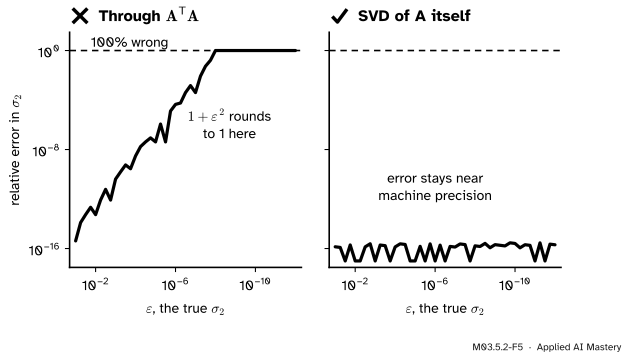
M03.5.2-F5
Wrong beside right. Through \(\mat{A}\T\mat{A}\) the small singular value loses accuracy fast and is lost entirely below \(\varepsilon \approx 10^{-8}\); the SVD of \(\mat{A}\) itself keeps it.
“To compute an SVD, form \(\mat{A}\T\mat{A}\) and take its eigenvectors.”
That is how we prove the SVD exists, not how to compute it. Forming \(\mat{A}\T\mat{A}\) squares every singular value, and a small one can sink below rounding error. Take the matrix with rows \((1, 1)\), \((\varepsilon, 0)\) and \((0, \varepsilon)\), with \(\varepsilon = 10^{-9}\). Its exact \(\mat{A}\T\mat{A}\) has diagonal entries \(1 + \varepsilon^2 = 1 + 10^{-18}\), which double precision stores as exactly \(1\). The stored matrix has rows \((1, 1)\) twice, whose smaller eigenvalue is exactly \(0\), so whatever tiny number the computer returns, \(\sigma_2 = 10^{-9}\) cannot be recovered from it. numpy.linalg.svd works on \(\mat{A}\) directly and finds it to about fifteen digits. Lesson M03.8.2 explains this as the condition number being squared.
“Take \(\mat{V}\) from \(\mat{A}\T\mat{A}\) and \(\mat{U}\) from \(\mat{A}\mat{A}\T\), separately.”
The \(\vect{u}_i\) are indeed eigenvectors of \(\mat{A}\mat{A}\T\), but an eigenvector is only fixed up to sign. Found independently, \(\vect{u}_1\) may come out as \(-(1, 3)/\sqrt{10}\) while \(\vect{v}_1 = (1, 1)/\sqrt{2}\), and then \(\mat{U}\mat{\Sigma}\mat{V}\T\) is not \(\mat{A}\). Compute \(\vect{u}_i = \mat{A}\vect{v}_i/\sigma_i\), which ties each sign to its partner.
“eigh lists the largest eigenvalue first.”
numpy.linalg.eigh returns eigenvalues in ascending order, while numpy.linalg.svd returns singular values in descending order. Forgetting to reverse gives \(\sigma_1 = \sqrt{5}\) and swaps the long and short axes of the ellipse.
Check yourself
Recall
1. How are the singular values of \(\mat{A}\) related to the eigenvalues of \(\mat{A}\T\mat{A}\)?
Show answer
They are their non-negative square roots: \(\sigma_i = \sqrt{\lambda_i}\).
2. Why are the eigenvalues of \(\mat{A}\T\mat{A}\) never negative?
Show answer
For a unit eigenvector, \(\lambda_i = \vect{v}_i\T\mat{A}\T\mat{A}\vect{v}_i = \norm{\mat{A}\vect{v}_i}^2 \ge 0\).
3. Once \(\vect{v}_i\) and \(\sigma_i > 0\) are known, how do you find \(\vect{u}_i\)?
Show answer
\(\vect{u}_i = \mat{A}\vect{v}_i / \sigma_i\).
4. What does \(\mat{A}\T\) do to \(\vect{u}_i\)?
Show answer
It sends it to \(\sigma_i\vect{v}_i\), because \(\mat{A}\T = \mat{V}\mat{\Sigma}\mat{U}\T\).
5. Why do library routines not compute an SVD by forming \(\mat{A}\T\mat{A}\)?
Show answer
Forming it squares the singular values, so small ones are lost to rounding; for example \(1 + 10^{-18}\) is stored as \(1\).
Exercises
1.★ Find the SVD of \(\mat{A} = \begin{bmatrix} 2 & 2 \\ 1 & -1 \end{bmatrix}\) through \(\mat{A}\T\mat{A}\).
Show solution
The columns are \((2, 1)\) and \((2, -1)\), so \(\mat{A}\T\mat{A}\) has entries \(4 + 1 = 5\), \(4 - 1 = 3\) and \(5\): rows \((5, 3)\) and \((3, 5)\). Trace \(10\), determinant \(16\), so \(\lambda^2 - 10\lambda + 16 = {(\lambda - 8)(\lambda - 2)}\). For \(\lambda = 8\), \(x = y\) and \(\vect{v}_1 = (1, 1)/\sqrt{2}\); for \(\lambda = 2\), \(y = -x\) and \(\vect{v}_2 = (1, -1)/\sqrt{2}\). So \(\sigma_1 = 2\sqrt{2}\) and \(\sigma_2 = \sqrt{2}\). Then \(\mat{A}\vect{v}_1 = (4, 0)/\sqrt{2}\), so \(\vect{u}_1 = (1, 0)\), and \(\mat{A}\vect{v}_2 = (0, 2)/\sqrt{2}\), so \(\vect{u}_2 = (0, 1)\). Check: \(\mat{U} = \mat{I}\), and \(\mat{\Sigma}\mat{V}\T\) has rows \({2\sqrt{2}\,(1, 1)/\sqrt{2}} = (2, 2)\) and \({\sqrt{2}\,(1, -1)/\sqrt{2}} = (1, -1)\), which is \(\mat{A}\).
2.★★ Show that \(\mat{A}\T\mat{A}\) and \(\mat{A}\mat{A}\T\) have the same non-zero eigenvalues, even when \(\mat{A}\) is not square.
Show solution
Let \(\mat{A}\T\mat{A}\vect{v} = \lambda\vect{v}\) with \(\vect{v} \ne \vect{0}\) and \(\lambda \ne 0\). Multiply on the left by \(\mat{A}\): \(\mat{A}\mat{A}\T(\mat{A}\vect{v}) = \lambda(\mat{A}\vect{v})\). The vector \(\mat{A}\vect{v}\) is not zero, because \(\norm{\mat{A}\vect{v}}^2 = \vect{v}\T\mat{A}\T\mat{A}\vect{v} = \lambda\norm{\vect{v}}^2 \ne 0\). So \(\lambda\) is an eigenvalue of \(\mat{A}\mat{A}\T\), with eigenvector \(\mat{A}\vect{v}\). The same argument with \(\mat{A}\T\) in place of \(\mat{A}\) gives the other direction. For the running \(\mat{A}\), \(\mat{A}\mat{A}\T\) has rows \((9, 12)\) and \((12, 41)\): trace \(50\), determinant \(225\), eigenvalues \(45\) and \(5\) again.
3.★★★ Let \(\mat{Q}\) be orthogonal. Prove that \(\mat{Q}\mat{A}\) and \(\mat{A}\mat{Q}\) have the same singular values as \(\mat{A}\), and say what that means for the ellipse.
Show solution
For \(\mat{Q}\mat{A}\): \({(\mat{Q}\mat{A})\T(\mat{Q}\mat{A})} = \mat{A}\T\mat{Q}\T\mat{Q}\mat{A} = \mat{A}\T\mat{A}\), the same matrix, so the same eigenvalues and singular values. For \(\mat{A}\mat{Q}\): \({(\mat{A}\mat{Q})\T(\mat{A}\mat{Q})} = \mat{Q}\T(\mat{A}\T\mat{A})\mat{Q}\). If \(\mat{A}\T\mat{A}\vect{v} = \lambda\vect{v}\), then \(\mat{Q}\T\mat{A}\T\mat{A}\mat{Q}(\mat{Q}\T\vect{v}) = \mat{Q}\T\mat{A}\T\mat{A}\vect{v} = \lambda\mat{Q}\T\vect{v}\), using \(\mat{Q}\mat{Q}\T = \mat{I}\), so \(\lambda\) is again an eigenvalue, with eigenvector \(\mat{Q}\T\vect{v}\). In pictures: turning the plane after \(\mat{A}\) turns the ellipse without changing its axes’ lengths, and turning before \(\mat{A}\) only relabels which inputs reach them.
Summary card
The right singular vectors are the eigenvectors of \(\mat{A}\T\mat{A}\), and \(\sigma_i^2\) are its eigenvalues.
M03.5.2-F1
The round trip keeps each \(\vect{v}_i\) on its line.
Key identity.\(\mat{A}\T\mat{A} = \mat{V}\mat{\Sigma}^2\mat{V}\T\), symmetric and semidefinite.
Recipe. Eigenvectors \(\vect{v}_i\), then \(\sigma_i = \sqrt{\lambda_i}\), then \(\vect{u}_i = \mat{A}\vect{v}_i/\sigma_i\).
Existence. The \(\vect{u}_i\) are orthonormal because \(\vect{v}_i\T\mat{A}\T\mat{A}\vect{v}_j = \lambda_j\,\vect{v}_i \cdot \vect{v}_j\).
Running example.\(\mat{A}\T\mat{A}\) has rows \((25, 20)\), \((20, 25)\); eigenvalues \(45\) and \(5\).
In practice. Call numpy.linalg.svd; never form \(\mat{A}\T\mat{A}\) for accuracy.
Sources and next steps
Sources. Each was opened and checked against this lesson on 15 November 2026.
Sheldon Axler, Linear Algebra Done Right, 4th edition, Section 7E: 7.64 (\(T^*T\) is a positive operator), 7.65 (singular values are the non-negative square roots of the eigenvalues of \(T^*T\)), 7.70 (the SVD, proved through the spectral theorem for \(T^*T\) and \(f_k = Te_k / s_k\), exactly the proof above) and 7.80 (the matrix version).
Marc Peter Deisenroth, A. Aldo Faisal and Cheng Soon Ong, Mathematics for Machine Learning, Section 4.5, equations (4.71) to (4.79): \(\mat{A}\T\mat{A} = \mat{V}\mat{\Sigma}\T\mat{\Sigma}\mat{V}\T\), \(\sigma_i^2 = \lambda_i\), the orthogonality of the \(\mat{A}\vect{v}_i\), and \(\vect{u}_i = \mat{A}\vect{v}_i/\sigma_i\).
David Austin, Understanding Linear Algebra, section “Singular value decompositions”: singular values as the square roots of the eigenvalues of the Gram matrix \(\mat{A}\T\mat{A}\), whose eigenvectors are the right singular vectors.
NumPy reference, numpy.linalg.eigh (eigenvalues in ascending order) and numpy.linalg.svd (singular values in descending order, Vh returned, full_matrices option).