A symmetric matrix equals its own mirror image across the diagonal. Prove that its eigenvalues are always real and that eigenvectors for different eigenvalues are always perpendicular, and meet the covariance, Gram, second-derivative and graph matrices where this matters.
M03.3.1L2 Intermediate25 minIn review (what this means)
The maths and code on this page are checked by automated tests on every change, but an independent reader has not signed it off yet. Spot a mistake or a confusing step? Tell us.
Recognise a symmetric matrix and name four places where machine learning produces one: covariance, Gram, second-derivative and graph matrices.
Prove the swap rule (Su) · v = u · (Sv) for a symmetric matrix S and use it to show that eigenvectors for distinct eigenvalues are perpendicular.
Prove that the eigenvalues of a real symmetric matrix are real, using complex conjugates.
Find the eigenvalues of [[a, b], [b, c]] from the discriminant (a - c)^2 + 4b^2 and explain why it is never negative.
The question
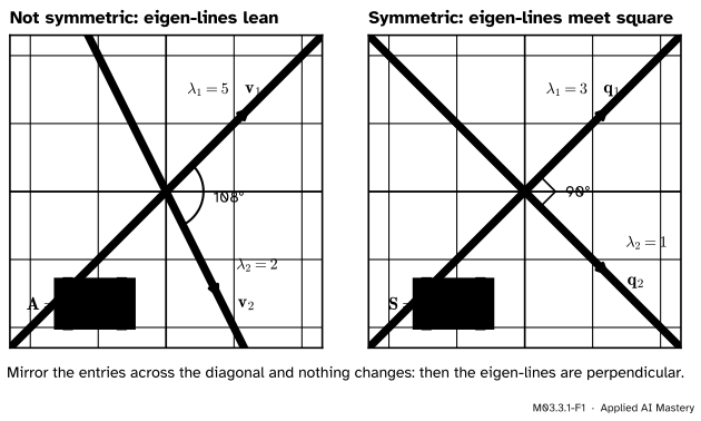
Ask principal component analysis for the main directions of a cloud of data and it always hands back directions at right angles to one another. Yet the eigenvectors of the running matrix \(\mat{A}\) of this course, \({(1, 1)}\) and \({(1, -2)}\), meet at about 108 degrees. What is special about the matrices that data science feeds to an eigenvalue routine, and why do their eigenvectors never lean?
Intuition
A matrix is symmetric when it equals its own mirror image across the main diagonal: the entry in row \(i\), column \(j\) equals the entry in row \(j\), column \(i\). The running matrix \(\mat{S} = \begin{bmatrix} 2 & 1 \\ 1 & 2 \end{bmatrix}\) is symmetric. The running matrix \(\mat{A} = \begin{bmatrix} 4 & 1 \\ 2 & 3 \end{bmatrix}\) is not, because its two off-diagonal entries are 1 and 2.
That small condition on the entries has a large effect on the picture.
M03.3.1-F1
The eigen-lines of the running matrix \(\mat{A}\) meet at about 108 degrees. Those of the symmetric \(\mat{S}\) meet at a right angle. Symmetry is what forces the right angle.
Two facts hold for every symmetric matrix with real entries, and this lesson proves both.
Its eigenvalues are real numbers. A symmetric matrix never turns the plane the way a rotation does, so it never needs the complex eigenvalues of lesson M03.1.4.
Eigenvectors for different eigenvalues are perpendicular. The directions the matrix keeps on their lines cross at right angles, as on the right of the figure.
Both facts come from one small identity, the swap rule, which you will meet in Step 2.
Build it up
Step 1. Where symmetric matrices come from. They are not rare. Almost every square matrix that a data scientist hands to an eigenvalue routine is symmetric, for one of four reasons.
M03.3.1-F2
Four sources of symmetric matrices. The shaded entries are mirror images of each other across the diagonal, and each card gives the reason they must be equal.
Covariance matrices. Lesson M06.10.2 put the variances of a pair of variables on the diagonal and their covariance off it. Covariance does not care about order, so the two off-diagonal entries agree.
Gram matrices. For any data matrix \(\mat{X}\), entry \(ij\) of \(\mat{X}\T\mat{X}\) is the dot product of column \(i\) with column \(j\), and a dot product does not care about order either. For the course’s running rectangular matrix \(\mat{B}\) with rows \({(1, 1)}\), \({(1, 0)}\) and \({(0, 1)}\), the two columns are \({(1, 1, 0)}\) and \({(1, 0, 1)}\), so \(\mat{B}\T\mat{B}\) has entries \({1 + 1 + 0} = 2\), \({1 + 0 + 0} = 1\), \(1\) and \(2\): it is \(\mat{S}\) itself.
Second partial derivatives. For the running bowl \({f(x, y)} = {2x^2 + 2xy + 2y^2}\), the partial derivatives of lesson M04.10.2 are \(\pd{f}{x} = {4x + 2y}\) and \(\pd{f}{y} = {2x + 4y}\). Differentiate each again. \({4x + 2y}\) has slope 4 in \(x\) and 2 in \(y\); \({2x + 4y}\) has slope 2 in \(x\) and 4 in \(y\). Arranged as a table, the four second derivatives are \(\begin{bmatrix} 4 & 2 \\ 2 & 4 \end{bmatrix} = 2\mat{S}\). The two mixed ones agree, here and for every function whose second derivatives are continuous (a theorem of course M05).
Undirected graphs. Put a 1 in row \(i\), column \(j\) when nodes \(i\) and \(j\) are joined. A friendship or a road runs both ways, so the table is symmetric.
Step 2. The swap rule. A symmetric matrix can jump from one side of a dot product to the other. Write the dot product as a row times a column, \({\vect{x} \cdot \vect{y}} = {\vect{x}\T\vect{y}}\), and recall that transposing a product reverses its order, \({(\mat{M}\vect{u})\T} = {\vect{u}\T\mat{M}\T}\). Then
The third line is the only place where symmetry is used: \(\mat{S}\T = \mat{S}\).
Check it with numbers. Take \(\vect{u} = {(1, 2)}\) and \(\vect{v} = {(3, -1)}\). Then \(\mat{S}\vect{u} = {(4, 5)}\) and \({(4, 5) \cdot (3, -1)} = {12 - 5} = 7\), while \(\mat{S}\vect{v} = {(5, 1)}\) and \({(1, 2) \cdot (5, 1)} = {5 + 2} = 7\). The same test on \(\mat{A}\) fails: \(\mat{A}\vect{u} = {(6, 8)}\) gives \({18 - 8} = 10\), but \(\mat{A}\vect{v} = {(11, 3)}\) gives \({11 + 6} = 17\).
Step 3. What the swap rule does to eigenvectors. Put two eigenvectors into the swap rule. On the left, \(\mat{S}\) acts on the first and turns into its eigenvalue; on the right, it acts on the second and turns into the other eigenvalue. The same dot product has been multiplied by two different numbers and yet stayed the same. That can only happen if the dot product is zero. The next section writes this out.
The formal statement
NoteDefinition and two theorems
A square matrix \(\mat{S}\) is symmetric if \(\mat{S}\T = \mat{S}\), that is, \(s_{ij} = s_{ji}\) for every \(i\) and \(j\). Let \(\mat{S}\) be a real symmetric matrix.
Perpendicular eigenvectors. If \(\mat{S}\vect{v}_1 = \lambda_1\vect{v}_1\) and \(\mat{S}\vect{v}_2 = \lambda_2\vect{v}_2\) with \({\lambda_1 \neq \lambda_2}\), then \({\vect{v}_1 \cdot \vect{v}_2} = 0\).
Real eigenvalues. Every eigenvalue of \(\mat{S}\) is a real number.
Proof of the first. Start from \({\lambda_1 (\vect{v}_1 \cdot \vect{v}_2)}\) and use each eigenvector equation once, with the swap rule in the middle:
Subtract the right end from the left end: \({(\lambda_1 - \lambda_2)(\vect{v}_1 \cdot \vect{v}_2)} = 0\). The first factor is not zero, because the eigenvalues differ. So the second factor is zero. \(\blacksquare\)
Proof of the second. An eigenvalue of a real matrix might be complex, with a complex eigenvector (lesson M03.1.4), so we must allow that. Suppose \(\mat{S}\vect{v} = \lambda\vect{v}\) with \({\vect{v} \neq \vect{0}}\), where \(\lambda\) and the entries of \(\vect{v}\) may be complex. Write \(\vect{v}^*\) for the vector of conjugates \(v_i^*\) (lesson M01.9). Three facts do the work.
Conjugating the equation entry by entry, and using that \(\mat{S}\) is real, gives \(\mat{S}\vect{v}^* = \lambda^*\vect{v}^*\).
For a complex number, \({z^* z} = \abs{z}^2\), so \({(\vect{v}^*)\T\vect{v}} = {\abs{v_1}^2 + \cdots + \abs{v_n}^2}\), which is a positive real number because some \(v_i\) is not zero.
Transposing \(\mat{S}\vect{v}^* = \lambda^*\vect{v}^*\), and using \(\mat{S}\T = \mat{S}\), gives \({(\vect{v}^*)\T\mat{S}} = {\lambda^* (\vect{v}^*)\T}\).
Now compute the number \({(\vect{v}^*)\T\mat{S}\vect{v}}\) in two ways. Grouping \(\mat{S}\vect{v}\) first and using the eigenvector equation:
The two right-hand sides are equal, and \({(\vect{v}^*)\T\vect{v}}\) is not zero (fact 2), so \(\lambda = \lambda^*\). A number equal to its own conjugate has imaginary part zero: \(\lambda\) is real. \(\blacksquare\)
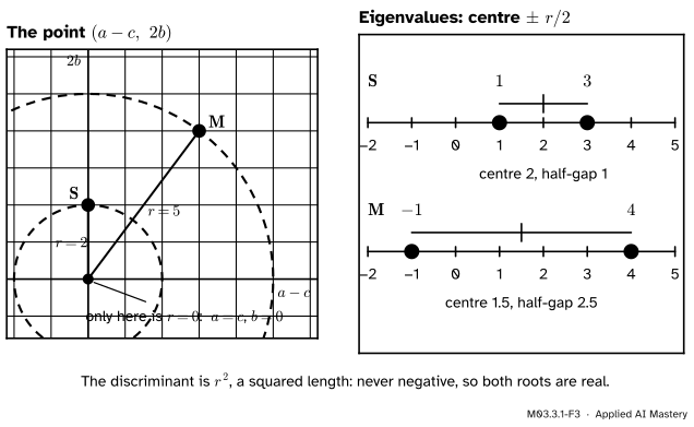
The 2 by 2 case in full. For \(\mat{S} = \begin{bmatrix} a & b \\ b & c \end{bmatrix}\) the characteristic polynomial of lesson M03.1.2 is \({\lambda^2 - (a + c)\lambda + (ac - b^2)}\). Its discriminant, “\({b^2 - 4ac}\)” of the quadratic formula, is
The discriminant is the squared distance \(r^2\) of the point \({(a - c,\; 2b)}\) from the origin. The two eigenvalues sit at the mean \({(a + c)/2}\) of the diagonal, \({r/2}\) either side of it.
The discriminant is zero only when \(a = c\) and \(b = 0\), that is, when \(\mat{S}\) is a multiple of the identity. Then the eigenvalue is repeated and every vector is an eigenvector. In every other case a real symmetric 2 by 2 matrix has two different real eigenvalues.
Go deeper: the eigenvectors of [[a, b], [b, c]], checked by hand
Suppose \({b \neq 0}\). For each root \(\lambda\), the vector \({(b,\; \lambda - a)}\) is an eigenvector. The first entry of \({\mat{S}\,(b,\; \lambda - a)}\) is \({ab + b(\lambda - a)} = {b\lambda}\), which is \(\lambda\) times \(b\). The second entry is \({b^2 + c(\lambda - a)}\), and it equals \({\lambda(\lambda - a)}\) exactly when \({\lambda^2 - (a + c)\lambda + ac - b^2} = 0\), which is true because \(\lambda\) is a root. For the two roots, the sum is \({\lambda_1 + \lambda_2} = {a + c}\) and the product is \(\lambda_1\lambda_2 = {ac - b^2}\) (lesson M03.1.3), so the dot product of the two eigenvectors is
Find the eigenvalues and eigenvectors of \(\mat{S} = \begin{bmatrix} 2 & 1 \\ 1 & 2 \end{bmatrix}\) and check that the eigenvectors are perpendicular.
M03.3.1-F4
The whole calculation for \(\mat{S}\), from the matrix to the zero dot product.
The polynomial. The trace is \({2 + 2} = 4\) and the determinant is \({4 - 1} = 3\), so the characteristic polynomial is \({\lambda^2 - 4\lambda + 3}\). Its discriminant is \({16 - 12} = 4\), which matches \({(a - c)^2 + 4b^2} = {0 + 4}\). It factors as \({(\lambda - 3)(\lambda - 1)}\), so \(\lambda_1 = 3\) and \(\lambda_2 = 1\).
The eigenvectors. For \(\lambda_1 = 3\), the first row of \({\mat{S} - 3\mat{I}}\) is \({(-1, 1)}\), so \({-x + y} = 0\) and \(\vect{v}_1 = {(1, 1)}\). For \(\lambda_2 = 1\), the first row of \({\mat{S} - \mat{I}}\) is \({(1, 1)}\), so \({x + y} = 0\) and \(\vect{v}_2 = {(1, -1)}\).
The check.\({\vect{v}_1 \cdot \vect{v}_2} = {1 - 1} = 0\). Divided by their length \({\sqrt{2}}\) they become the course’s orthonormal pair \({\vect{q}_1 = (1, 1)/\sqrt{2}}\) and \({\vect{q}_2 = (1, -1)/\sqrt{2}}\).
A second matrix, by the formula. Take \(\mat{M} = \begin{bmatrix} 3 & 2 \\ 2 & 0 \end{bmatrix}\), so \(a = 3\), \(b = 2\), \(c = 0\). The discriminant is \({(3 - 0)^2 + 4 \cdot 4} = 25\), so
\[
\lambda = \frac{3}{2} \pm \frac{5}{2}, \quad\text{that is, } 4 \text{ or } -1 .
\]
The vectors \({(b,\; \lambda - a)}\) are \({(2, 1)}\) for \(\lambda = 4\) and \({(2, -4)}\) for \(\lambda = {-1}\); the second is a multiple of \({(1, -2)}\). Check by multiplying: \({\mat{M}\,(2, 1)} = {(6 + 2,\; 4 + 0)} = {(8, 4)} = {4\,(2, 1)}\) and \({\mat{M}\,(1, -2)} = {(3 - 4,\; 2 + 0)} = {(-1, 2)} = {-1\,(1, -2)}\). The dot product is \({2 \cdot 1 + 1 \cdot (-2)} = 0\). One eigenvalue is negative, and that is allowed: symmetry promises real eigenvalues, not positive ones.
Code
From scratch: the 2 by 2 formula, then the swap rule and both theorems tested on many random matrices.
import mathimport numpy as npdef eig_sym2(a, b, c):"""Eigenvalues (larger first) and eigenvectors of [[a, b], [b, c]], from the formula.""" centre, half = (a + c) /2, math.sqrt((a - c) **2+4* b **2) /2 lams = (centre + half, centre - half)if b ==0: # already diagonal: the axes are eigenvectors vecs = ((1.0, 0.0), (0.0, 1.0)) if a >= c else ((0.0, 1.0), (1.0, 0.0))else: vecs =tuple((b, lam - a) for lam in lams)return lams, vecsfor name, (a, b, c) in {"S": (2, 1, 2), "M": (3, 2, 0)}.items(): lams, (v1, v2) = eig_sym2(a, b, c)print(name, "eigenvalues", lams, " eigenvectors", v1, v2," dot", v1[0] * v2[0] + v1[1] * v2[1])
Now ten thousand random symmetric matrices, each made as \({(\mat{M} + \mat{M}\T)/2}\) from a random \(\mat{M}\), beside ten thousand random matrices with no symmetry at all.
rng = np.random.default_rng(0)u, v = np.array([1.0, 2.0]), np.array([3.0, -1.0])S = np.array([[2.0, 1.0], [1.0, 2.0]])A = np.array([[4.0, 1.0], [2.0, 3.0]])print("swap rule for S:", (S @ u) @ v, u @ (S @ v), " for A:", (A @ u) @ v, u @ (A @ v))complex_sym = complex_any =0worst_dot =0.0for _ inrange(10_000): M = rng.normal(size=(3, 3)) sym = (M + M.T) /2 lams = np.linalg.eigvals(sym) complex_sym += np.any(np.abs(lams.imag) >1e-12) complex_any += np.any(np.abs(np.linalg.eigvals(M).imag) >1e-12) _, vecs = np.linalg.eigh(sym) # columns are eigenvectors worst_dot =max(worst_dot, abs(vecs[:, 0] @ vecs[:, 1]))print("symmetric with complex eigenvalues:", complex_sym, "of 10000")print("unsymmetric with complex eigenvalues:", complex_any, "of 10000")print("largest |q1 . q2| over all symmetric ones:", worst_dot)
swap rule for S: 7.0 7.0   for A: 10.0 17.0
symmetric with complex eigenvalues: 0 of 10000
unsymmetric with complex eigenvalues: 6492 of 10000
largest |q1 . q2| over all symmetric ones: 8.326672684688674e-16
Not one symmetric matrix produced a complex eigenvalue, and every pair of eigenvectors that eigh returned was perpendicular to within rounding. About 65 in every 100 of the unsymmetric 3 by 3 matrices had a complex pair. (Rounding error is the only reason the largest dot product is not exactly 0.)
NumPy has a routine made for symmetric matrices: np.linalg.eigvalsh for the eigenvalues alone and np.linalg.eigh for eigenvalues and eigenvectors. Both return the eigenvalues as real numbers in ascending order. Here they are on the four matrices of the figure in Step 1.
The covariance matrix is \({\mat{S}/4}\) and the matrix of second derivatives is \(2\mat{S}\), so their eigenvalues are those of \(\mat{S}\), 3 and 1, scaled by \({\tfrac14}\) and by 2. The path graph has eigenvalues \({-\sqrt{2}}\), 0 and \({\sqrt{2}}\): real, and one of them negative.
Explore
This module’s interactive, the spectral ellipse, lives in lesson M03.3.2. Its three sliders set the entries \(a\), \(b\) and \(c\) of a symmetric matrix. However you set them, the two eigenvector arrows stay at a right angle. Set \(b = 0\) and \(a = c\) to see the one case where the eigenvalues meet.
Pitfalls
M03.3.1-F5
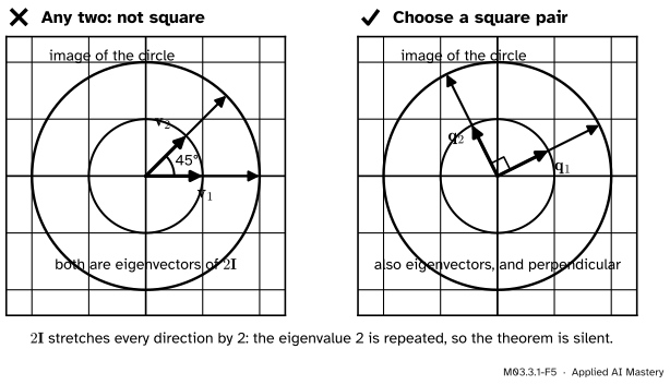
Wrong beside right. With a repeated eigenvalue, two eigenvectors can lean. The theorem only promises a right angle for different eigenvalues, so a perpendicular pair has to be chosen.
“Every two eigenvectors of a symmetric matrix are perpendicular.”
Only when their eigenvalues differ. The matrix \(2\mat{I}\) is symmetric, and \({(1, 0)}\) and \({(1, 1)}\) are both eigenvectors of it, at 45 degrees. When an eigenvalue repeats, its eigenvectors fill a whole plane (or more), and some pairs in it lean. The next lesson shows that a perpendicular pair can always be chosen, with Gram-Schmidt.
“Its eigenvalues are real, so the matrix must be symmetric.”
The running matrix \(\mat{A}\) has the real eigenvalues 5 and 2, but it is not symmetric, and its eigenvectors lean at 108 degrees (the left of the first figure). Symmetry is enough for real eigenvalues; it is not needed for them.
“A symmetric matrix has positive eigenvalues.”
Real, yes; positive, no. The matrix \(\mat{M}\) of the worked example has the eigenvalue \({-1}\), and the running saddle \(\begin{bmatrix} 1 & 2 \\ 2 & 1 \end{bmatrix}\) has 3 and \({-1}\). The symmetric matrices with only positive eigenvalues are special enough to have their own module, M03.4.
Check yourself
Recall
1. What does it mean for a matrix to be symmetric, entry by entry?
Show answer
\(s_{ij} = s_{ji}\) for all \(i\) and \(j\): the matrix equals its mirror image across the main diagonal, \(\mat{S}\T = \mat{S}\).
2. State the swap rule, and say where symmetry enters its proof.
Show answer
\({(\mat{S}\vect{u}) \cdot \vect{v}} = {\vect{u} \cdot (\mat{S}\vect{v})}\). Writing the left side as \({\vect{u}\T\mat{S}\T\vect{v}}\), symmetry replaces \(\mat{S}\T\) by \(\mat{S}\).
3. Why must eigenvectors for different eigenvalues of a symmetric matrix be perpendicular?
Show answer
By the swap rule, \({\lambda_1 (\vect{v}_1 \cdot \vect{v}_2)} = {\lambda_2 (\vect{v}_1 \cdot \vect{v}_2)}\). Since \({\lambda_1 \neq \lambda_2}\), the dot product must be zero.
4. What is the discriminant of the characteristic polynomial of \(\begin{bmatrix} a & b \\ b & c \end{bmatrix}\), and why is it never negative?
Show answer
\({(a - c)^2 + 4b^2}\). It is a sum of two squares.
5. Name two places in machine learning where symmetric matrices come from, and the reason each is symmetric.
Show answer
Any two of: covariance matrices (covariance does not care about order), Gram matrices \(\mat{X}\T\mat{X}\) (a dot product does not care about order), matrices of second partial derivatives (the mixed partials agree) and adjacency matrices of undirected graphs (an edge runs both ways).
Exercises
1.★ Which of these are symmetric? Compute the third. (a) \(\begin{bmatrix} 1 & 4 \\ 4 & -2 \end{bmatrix}\) (b) \(\begin{bmatrix} 0 & -1 \\ 1 & 0 \end{bmatrix}\) (c) \(\mat{X}\T\mat{X}\) for the matrix \(\mat{X}\) with rows \({(1, 2)}\), \({(0, 1)}\) and \({(1, 0)}\).
Show solution
(a) Symmetric: both off-diagonal entries are 4.
(b) Not symmetric: the off-diagonal entries are \({-1}\) and \(1\). (It is the turn by 90 degrees, with eigenvalues \(i\) and \({-i}\), which shows that without symmetry the eigenvalues need not be real.)
(c) The columns of \(\mat{X}\) are \({(1, 0, 1)}\) and \({(2, 1, 0)}\). The entries of \(\mat{X}\T\mat{X}\) are their dot products: \({1 + 0 + 1} = 2\), \({2 + 0 + 0} = 2\), again \(2\), and \({4 + 1 + 0} = 5\). So \(\mat{X}\T\mat{X} = \begin{bmatrix} 2 & 2 \\ 2 & 5 \end{bmatrix}\), which is symmetric, as every Gram matrix is.
2.★★ Find the eigenvalues and eigenvectors of the running saddle \(\begin{bmatrix} 1 & 2 \\ 2 & 1 \end{bmatrix}\) with the formula of this lesson, and check that the eigenvectors are perpendicular.
Show solution
Here \(a = c = 1\) and \(b = 2\). The discriminant is \({0 + 4 \cdot 4} = 16\), so
\[
\lambda = \frac{2}{2} \pm \frac{4}{2}, \quad\text{that is, } 3 \text{ or } -1 .
\]
The vectors \({(b,\; \lambda - a)}\) are \({(2, 2)}\) for \(\lambda = 3\) and \({(2, -2)}\) for \(\lambda = {-1}\), multiples of \({(1, 1)}\) and \({(1, -1)}\). Check: the matrix sends \({(1, 1)}\) to \({(3, 3)}\) and \({(1, -1)}\) to \({(-1, 1)}\). The dot product is \({1 - 1} = 0\). The saddle has the same eigenvectors as \(\mat{S}\), because both are of the form \({p\mat{I} + q\begin{bmatrix} 0 & 1 \\ 1 & 0 \end{bmatrix}}\).
3.★★★ Let \(\mat{S}\) be symmetric and let \(\vect{u}\) be an eigenvector, \(\mat{S}\vect{u} = \lambda\vect{u}\). Show that if \(\vect{w}\) is perpendicular to \(\vect{u}\), then so is \(\mat{S}\vect{w}\). Deduce that a symmetric 2 by 2 matrix with one eigenvector has a second one perpendicular to it.
So \(\mat{S}\) sends the set of vectors perpendicular to \(\vect{u}\) into itself. In the plane that set is a single line, spanned by one non-zero vector \(\vect{w}\). Since \(\mat{S}\vect{w}\) lies on the same line, \(\mat{S}\vect{w} = \mu\vect{w}\) for some number \(\mu\): the vector \(\vect{w}\) is a second eigenvector, perpendicular to the first. The next lesson builds the spectral theorem on exactly this argument.
Summary card
Symmetric means real eigenvalues and perpendicular eigenvectors.
M03.3.1-F1
Mirror-equal entries, square eigen-lines.
Symmetric.\(\mat{S}\T = \mat{S}\), that is \(s_{ij} = s_{ji}\).
Sources. Each was opened and checked against this lesson on 15 November 2026.
Gilbert Strang, Symmetric matrices and positive definiteness, MIT OpenCourseWare 18.06SC, lecture 25 and its lecture summary. The summary states that a real symmetric matrix has real eigenvalues and perpendicular eigenvectors, and proves the eigenvalues real by conjugating \(\mat{A}\vect{x} = \lambda\vect{x}\), transposing, and computing the same product two ways, the argument used here (Strang writes the conjugate with a bar over the letter).
David Austin, Understanding Linear Algebra, Symmetric matrices and variance (open textbook). States that the eigenvalues of a symmetric matrix are real and that eigenvectors for different eigenvalues are orthogonal, and works with covariance matrices.
Sheldon Axler, Linear Algebra Done Right, 4th edition (open access). Result 7.12: every eigenvalue of a self-adjoint operator is real. Result 7.22: eigenvectors of a normal operator for distinct eigenvalues are orthogonal, by the same chain of equalities as here. On \(\R^n\) with the dot product, a self-adjoint operator is one with a symmetric matrix, and self-adjoint operators are normal.
Marc Peter Deisenroth, A. Aldo Faisal and Cheng Soon Ong, Mathematics for Machine Learning (free PDF). Theorem 4.14: \(\mat{A}\T\mat{A}\) is symmetric for every matrix \(\mat{A}\). Theorem 4.15, the spectral theorem, includes that each eigenvalue of a symmetric matrix is real.
NumPy reference, numpy.linalg.eigh and numpy.linalg.eigvalsh. For a real symmetric matrix they return the eigenvalues in ascending order, and eigh the normalised eigenvectors as columns.
Next.M03.3.2 The spectral theorem shows that a symmetric matrix always has a full set of perpendicular unit eigenvectors, even when an eigenvalue repeats, and reads \(\mat{S} = \mat{Q}\mat{\Lambda}\mat{Q}\T\) as turn, stretch, turn back.