Put the eigenvectors of a matrix in the columns of P and its eigenvalues on the diagonal of D. Derive A P = P D column by column, so that A = P D P inverse, work it by hand for the running matrix, and see which matrices cannot be taken apart this way.
M03.2.1L2 Intermediate25 minIn review (what this means)
The maths and code on this page are checked by automated tests on every change, but an independent reader has not signed it off yet. Spot a mistake or a confusing step? Tell us.
Derive A P = P D column by column from the eigenvector equations, and turn it into A = P D P^(-1) and P^(-1) A P = D.
Diagonalise a 2 by 2 matrix by hand and check the factorisation by multiplying it back together.
Decide whether a matrix is diagonalisable by counting independent eigenvectors, using distinct eigenvalues as a quick sufficient test.
Explain why the shear cannot be diagonalised and why a rotation can be diagonalised only with complex numbers.
The question
In lesson M02.9.4 a trick that works for \(\mat{S}\) found a basis in which its matrix became diagonal: a stretch along one line, a stretch along another, nothing else. Module M03.1 then gave a method that finds eigenvectors for any matrix. Put the two together. Can every matrix be written as “change to a good basis, stretch, change back”, and what exactly do the three pieces look like? The answer is the factorisation behind fast matrix powers, Markov chains, PageRank and principal component analysis.
with eigenvalues 5 and 2 and eigenvectors \(\vect{v}_1 = (1, 1)\) and \(\vect{v}_2 = (1, -2)\) (module M03.1). Each eigenvector stays on its own line: \(\mat{A}\) stretches \(\vect{v}_1\) by 5 and \(\vect{v}_2\) by 2.
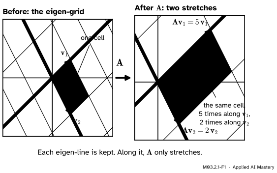
Now build a grid out of the two eigenvectors instead of out of \(\ihat\) and \(\jhat\). Every grid line runs along \(\vect{v}_1\) or along \(\vect{v}_2\). When \(\mat{A}\) acts, each of those lines lands on a line in the same direction. Nothing turns. The grid is only stretched: five times along one family of lines and twice along the other.
M03.2.1-F1
On the grid made of its eigenvectors, \(\mat{A}\) does nothing but stretch: by 5 along \(\vect{v}_1\) and by 2 along \(\vect{v}_2\). The same matrix on the square grid turns every arrow that is not an eigenvector.
So in the coordinates of this grid, \(\mat{A}\) is the diagonal matrix with entries 5 and 2. To use that, we need two translations: from ordinary coordinates into eigen-coordinates, and back. The matrix whose columns are the eigenvectors does the second job, and its inverse does the first. That is the whole idea of diagonalisation.
This is the change-of-basis matrix of lesson M02.9.2 for the basis of eigenvectors.
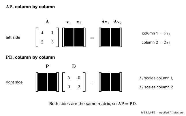
Step 3. Multiply \(\mat{A}\) by \(\mat{P}\), one column at a time. Column \(j\) of a product \(\mat{A}\mat{P}\) is \(\mat{A}\) times column \(j\) of \(\mat{P}\) (lesson M02.5). So the columns of \(\mat{A}\mat{P}\) are \(\mat{A}\vect{v}_1\) and \(\mat{A}\vect{v}_2\), and by Step 1 these are \(5\,\vect{v}_1\) and \(2\,\vect{v}_2\).
Step 4. Recognise the same matrix as a product the other way round. Put the eigenvalues on the diagonal of
Column \(j\) of \(\mat{P}\mat{D}\) is \(\mat{P}\) times column \(j\) of \(\mat{D}\). Column 1 of \(\mat{D}\) is \({(5, 0)}\), so the first column of \(\mat{P}\mat{D}\) is \({5\,\vect{v}_1 + 0\,\vect{v}_2} = 5\,\vect{v}_1\). Column 2 is \({(0, 2)}\), giving \(2\,\vect{v}_2\). Multiplying by a diagonal matrix on the right scales the columns.
M03.2.1-F2
Both products have the columns \(5\,\vect{v}_1\) and \(2\,\vect{v}_2\), so they are equal. The eigenvector equations, written side by side, are the single matrix equation \(\mat{A}\mat{P} = \mat{P}\mat{D}\).
Step 5. Undo \(\mat{P}\). The columns \((1, 1)\) and \((1, -2)\) are not on one line, so \(\mat{P}\) has an inverse. Multiply \(\mat{A}\mat{P} = \mat{P}\mat{D}\) on the right by \(\mat{P}^{-1}\):
The second form is the rule of lesson M02.9.3 for the matrix of a map in a new basis. In the basis of eigenvectors, the matrix of \(\mat{A}\) is \(\mat{D}\).
The formal statement
NoteTheorem: diagonalisation
An \({n \times n}\) matrix \(\mat{A}\) is diagonalisable if there are an invertible matrix \(\mat{P}\) and a diagonal matrix \(\mat{D}\) with \(\mat{A} = \mat{P}\mat{D}\mat{P}^{-1}\).
\(\mat{A}\) is diagonalisable exactly when it has \(n\) independent eigenvectors. The columns of \(\mat{P}\) are then those eigenvectors, and the diagonal of \(\mat{D}\) holds their eigenvalues, in the same order.
Proof.If \(\mat{A}\) has \(n\) independent eigenvectors. Call them \(\vect{v}_1, \dots, \vect{v}_n\), with \(\mat{A}\vect{v}_j = \lambda_j\vect{v}_j\). Put them in the columns of \(\mat{P}\) and let \(\mat{D}\) have diagonal \(\lambda_1, \dots, \lambda_n\). Column \(j\) of \(\mat{A}\mat{P}\) is \(\mat{A}\vect{v}_j = \lambda_j\vect{v}_j\). Column \(j\) of \(\mat{D}\) is \(\lambda_j\vect{e}_j\), so column \(j\) of \(\mat{P}\mat{D}\) is \({\mat{P}(\lambda_j\vect{e}_j)} = \lambda_j\vect{v}_j\). The columns agree, so \(\mat{A}\mat{P} = \mat{P}\mat{D}\). Independent columns make \(\mat{P}\) invertible (M02.7), and multiplying on the right by \(\mat{P}^{-1}\) gives \(\mat{A} = \mat{P}\mat{D}\mat{P}^{-1}\).
If \(\mat{A} = \mat{P}\mat{D}\mat{P}^{-1}\). Multiply on the right by \(\mat{P}\) to get \(\mat{A}\mat{P} = \mat{P}\mat{D}\). Comparing column \(j\) of each side, as above, \(\mat{A}\vect{p}_j = d_j\vect{p}_j\), where \(\vect{p}_j\) is column \(j\) of \(\mat{P}\) and \(d_j\) the diagonal entry. An invertible matrix has no zero column, so each \(\vect{p}_j\) is an eigenvector, and its columns are independent. That is \(n\) independent eigenvectors. \(\blacksquare\)
The picture of the theorem is three moves, read from the right of \(\mat{P}\mat{D}\mat{P}^{-1}\).
M03.2.1-F5
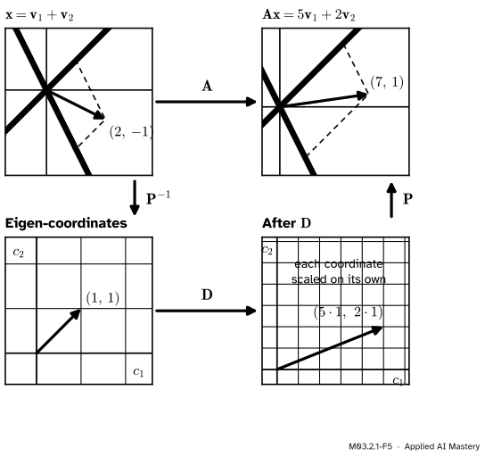
Two routes from \(\vect{x}\) to \(\mat{A}\vect{x}\). Across the top: multiply by \(\mat{A}\). The long way round: \(\mat{P}^{-1}\) finds the eigen-coordinates \((1, 1)\), \(\mat{D}\) scales each one on its own, and \(\mat{P}\) turns the result back into ordinary coordinates.
When is a matrix diagonalisable? Lesson M03.1.3 proved that eigenvectors for different eigenvalues are independent. So an \({n \times n}\) matrix with \(n\)distinct eigenvalues is always diagonalisable: one eigenvector from each eigenvalue already gives \(n\) independent ones. Distinct eigenvalues are enough but not necessary. The identity has the eigenvalue 1 twice, yet every vector is an eigenvector, and \(\mat{I} = \mat{I}\,\mat{I}\,\mat{I}^{-1}\) is diagonalised already. The trouble comes only when a repeated eigenvalue has too few eigenvectors.
Two ways to fail.
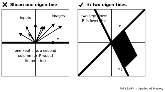
The shear\(\begin{bmatrix} 1 & 1 \\ 0 & 1 \end{bmatrix}\) has the eigenvalue 1 twice. Its eigenvectors solve \({(\mat{A} - \mat{I})}\vect{v} = \vect{0}\), that is, \(v_2 = 0\): only the horizontal line. Any two eigenvectors are multiples of \((1, 0)\), so no invertible \(\mat{P}\) can be built. The shear is defective: not diagonalisable at all.
The rotation by 90 degrees\(\mat{R} = \begin{bmatrix} 0 & -1 \\ 1 & 0 \end{bmatrix}\) keeps no real line, so no real \(\mat{P}\) exists. But it has the complex eigenvalues \(i\) and \(-i\) (lesson M03.1.4), and \({\mat{R}(1, -i)} = {(i, 1)} = {i\,(1, -i)}\). With complex eigenvectors \(\mat{R}\) does diagonalise:
So “diagonalisable” always comes with a choice of numbers. Over the real numbers \(\mat{R}\) is not diagonalisable; over the complex numbers it is.
Worked example
Diagonalise \(\mat{A} = \begin{bmatrix} 4 & 1 \\ 2 & 3 \end{bmatrix}\) and check the result by multiplying it back together.
Eigenvalues. The trace is 7 and the determinant \({4 \cdot 3} - {1 \cdot 2} = 10\), so the characteristic polynomial is \({\lambda^2 - 7\lambda + 10} = {(\lambda - 5)(\lambda - 2)}\). They are distinct, so \(\mat{A}\) is diagonalisable.
Eigenvectors. For \(\lambda = 5\), \(\mat{A} - 5\mat{I}\) has first row \({(-1, 1)}\), so \({-v_1 + v_2} = 0\) and \(\vect{v}_1 = (1, 1)\). For \(\lambda = 2\), the first row of \(\mat{A} - 2\mat{I}\) is \({(2, 1)}\), so \({2v_1 + v_2} = 0\) and \(\vect{v}_2 = (1, -2)\).
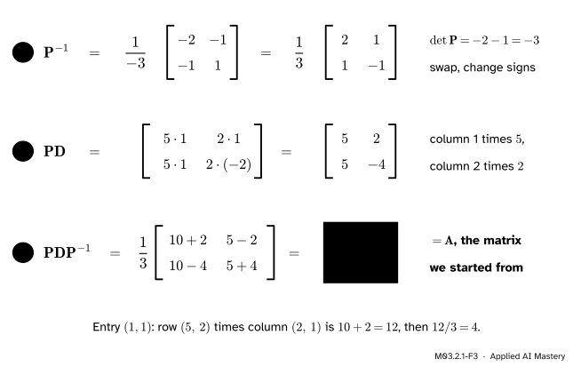
The three factors.\(\mat{P}\) has columns \(\vect{v}_1\), \(\vect{v}_2\) and \(\mat{D}\) has diagonal 5, 2. For the inverse, use the 2 by 2 rule: swap the diagonal entries, change the sign of the other two, divide by the determinant \({1 \cdot (-2)} - {1 \cdot 1} = -3\).
M03.2.1-F3
The check by hand. \(\mat{D}\) scales the columns of \(\mat{P}\), and multiplying by \(\mat{P}^{-1}\) returns exactly the matrix we started from.
Check: \({\mat{P}\mat{P}^{-1}}\) has entry \((1, 1)\) equal to \({\tfrac13(1 \cdot 2 + 1 \cdot 1)} = 1\) and entry \((2, 1)\) equal to \({\tfrac13(1 \cdot 2 + (-2) \cdot 1)} = 0\), and the other two entries work the same way.
Step 2: \(\mat{P}\mat{D}\) scales column 1 of \(\mat{P}\) by 5 and column 2 by 2. Step 3 multiplies row by column:
Use it on a vector. Take \(\vect{x} = (2, -1)\). Its eigen-coordinates are \({\mat{P}^{-1}\vect{x}} = {\tfrac13(4 - 1,\; 2 + 1)} = (1, 1)\), so \(\vect{x} = \vect{v}_1 + \vect{v}_2\). \(\mat{D}\) turns them into \((5, 2)\), and \(\mat{P}\) turns those back into \({5\,(1, 1) + 2\,(1, -2)} = (7, 1)\). Directly, \({\mat{A}\vect{x}} = {(8 - 1,\; 4 - 3)} = (7, 1)\). That is the route in the square of four panels above.
Code
From scratch first. The eigenvalues come from the quadratic formula of lesson M03.1.2, and for a matrix \({\begin{bmatrix} a & b \\ c & d \end{bmatrix}}\) with \(b \neq 0\), the vector \({(b,\; \lambda - a)}\) is an eigenvector: its first row gives \({a b + b(\lambda - a)} = \lambda b\), and its second row gives \(\lambda\) times \({(\lambda - a)}\) because \(\lambda\) is a root of the characteristic polynomial. Exact fractions keep every entry exact.
import mathfrom fractions import Fractiondef eig2(M):"""Eigenvalues (larger first) and eigenvectors of a 2 by 2 matrix with real eigenvalues and b != 0.""" (a, b), (c, d) = M tr, det = a + d, a * d - b * c root = math.isqrt(tr * tr -4* det) # exact when the discriminant is a perfect squareassert root * root == tr * tr -4* det lams = [Fraction(tr + root, 2), Fraction(tr - root, 2)]return lams, [(b, lam - a) for lam in lams]def matmul(X, Y):return [[sum(X[i][k] * Y[k][j] for k inrange(2)) for j inrange(2)] for i inrange(2)]def inverse2(M): (p, q), (r, s) = M det = Fraction(p * s - q * r)return [[s / det, -q / det], [-r / det, p / det]]A = [[4, 1], [2, 3]]lams, vecs = eig2(A)P = [[vecs[0][0], vecs[1][0]], [vecs[0][1], vecs[1][1]]] # eigenvectors as columnsD = [[lams[0], 0], [0, lams[1]]]rebuilt = matmul(matmul(P, D), inverse2(P))print("eigenvalues:", [str(l) for l in lams], " eigenvectors:", [tuple(map(int, v)) for v in vecs])print("P D P^-1 =", [[str(e) for e in row] for row in rebuilt])
eigenvalues: ['5', '2']   eigenvectors: [(1, 1), (1, -2)]
P D P^-1 = [['4', '1'], ['2', '3']]
The function’s eigenvectors are \((1, 1)\) and \((1, -2)\) exactly, because for this matrix \(b = 1\). Now NumPy. np.linalg.eig returns the eigenvalues and a matrix whose columns are eigenvectors scaled to length 1; the order of the eigenvalues and the sign of each column are not promised.
import numpy as npA = np.array([[4.0, 1.0], [2.0, 3.0]])w, V = np.linalg.eig(A)print("eigenvalues:", w)print("columns of V:\n", V.round(4))print("A V - V D =\n", (A @ V - V @ np.diag(w)).round(12) +0.0)print("V D V^-1 =\n", (V @ np.diag(w) @ np.linalg.inv(V)).round(12) +0.0)
eigenvalues: [5.+0.j 2.+0.j]
columns of V:
 [[ 0.7071+0.j -0.4472+0.j]
 [ 0.7071+0.j  0.8944+0.j]]
A V - V D =
 [[0.+0.j 0.+0.j]
 [0.+0.j 0.+0.j]]
V D V^-1 =
 [[4.+0.j 1.+0.j]
 [2.+0.j 3.+0.j]]
NumPy’s columns are our eigenvectors divided by their lengths, \(\sqrt2\) and \(\sqrt5\), possibly with a sign flipped. Any non-zero multiple of an eigenvector is an eigenvector, and exercise 3 shows that rescaling the columns of \(\mat{P}\) never changes \(\mat{P}\mat{D}\mat{P}^{-1}\).
Last, the two failures. For the shear NumPy still returns two columns, but they lie on one line, so the “inverse” does not exist in any useful sense. For the rotation the eigenvalues and eigenvectors are complex, and the factorisation works.
shear = np.array([[1.0, 1.0], [0.0, 1.0]])w_s, V_s = np.linalg.eig(shear)print("shear eigenvalues:", w_s.real, " det of its V:", np.linalg.det(V_s.real))R = np.array([[0.0, -1.0], [1.0, 0.0]])w_r, V_r = np.linalg.eig(R)print("rotation eigenvalues:", w_r)print("V D V^-1 =\n", (V_r @ np.diag(w_r) @ np.linalg.inv(V_r)).real.round(12) +0.0)
shear eigenvalues: [1. 1.]   det of its V: 2.2204460492503185e-16
rotation eigenvalues: [0.+1.j 0.-1.j]
V D V^-1 =
 [[ 0. -1.]
 [ 1.  0.]]
The determinant of the shear’s eigenvector matrix comes out around \(10^{-16}\) (the exact digits depend on the machine), where an honest basis would give a number of ordinary size: NumPy’s two “eigenvectors” are the same line, and rounding alone keeps them apart.
Explore
This module’s interactive, the power stepper, lives in lesson M03.2.2. Choose the running matrix \(\mat{A}\) and look at the bars: they show the two eigen-coordinates of the vector, the numbers \(\mat{P}^{-1}\) produces in this lesson. Press step once and check that the first bar is multiplied by 5 and the second by 2.
Pitfalls
M03.2.1-F4
Wrong beside right. The shear keeps only one line, so its eigenvectors cannot fill the two columns of an invertible \(\mat{P}\). The running matrix keeps two lines, and they span the plane.
“A repeated eigenvalue means the matrix cannot be diagonalised.”
Not always. The identity has the eigenvalue 1 twice and is already diagonal. What matters is whether the repeated eigenvalue has as many independent eigenvectors as its multiplicity (its eigenspace is big enough, lesson M03.1.3). The shear has the eigenvalue 1 twice but only one line of eigenvectors, and that is the failure.
“Diagonalisable and invertible mean the same thing.”
They are separate questions. \(\begin{bmatrix} 1 & 1 \\ 1 & 1 \end{bmatrix}\) has eigenvalues 2 and 0 with eigenvectors \((1, 1)\) and \((1, -1)\), so it is diagonalisable, but the eigenvalue 0 makes it singular. The shear is invertible (determinant 1) and not diagonalisable. Invertibility asks about \(\mat{A}\); diagonalisability asks about \(\mat{P}\).
“The order inside \(\mat{P}\) and \(\mat{D}\) does not matter.”
Each order is allowed, but the two must match. Swap the columns of \(\mat{P}\) without swapping the diagonal of \(\mat{D}\) and the product is a different matrix: with columns \((1, -2)\), \((1, 1)\) and diagonal 5, 2, \(\mat{P}\mat{D}\mat{P}^{-1}\) comes out as \(\begin{bmatrix} 3 & -1 \\ -2 & 4 \end{bmatrix}\), not \(\mat{A}\). NumPy pairs column \(j\) of V with entry \(j\) of w; keep them together.
Check yourself
Recall
1. What goes into the columns of \(\mat{P}\) and onto the diagonal of \(\mat{D}\)?
Show answer
The eigenvectors of \(\mat{A}\) go into the columns of \(\mat{P}\), and their eigenvalues, in the same order, onto the diagonal of \(\mat{D}\).
2. Why does \(\mat{A}\mat{P} = \mat{P}\mat{D}\) hold?
Show answer
Column \(j\) of \(\mat{A}\mat{P}\) is \(\mat{A}\vect{v}_j = \lambda_j\vect{v}_j\), and column \(j\) of \(\mat{P}\mat{D}\) is \(\mat{P}\) times \(\lambda_j\vect{e}_j\), which is also \(\lambda_j\vect{v}_j\).
3. When is an \(n \times n\) matrix diagonalisable?
Show answer
Exactly when it has \(n\) independent eigenvectors. Having \(n\) distinct eigenvalues is enough to guarantee that.
4. What are \(\mat{P}\), \(\mat{D}\) and \(\mat{P}^{-1}\) for the running matrix \(\mat{A}\)?
5. Why can the shear \(\begin{bmatrix} 1 & 1 \\ 0 & 1 \end{bmatrix}\) not be diagonalised?
Show answer
Its only eigenvalue is 1 and its eigenvectors all lie on the horizontal line, so there are not two independent eigenvectors to make an invertible \(\mat{P}\).
\(\mat{B}\) is triangular, so its eigenvalues are its diagonal entries, 2 and 3. For \(\lambda = 2\), \(\mat{B} - 2\mat{I}\) has second row \({(1, 1)}\), so \({v_1 + v_2} = 0\) and \(\vect{v}_1 = (1, -1)\). For \(\lambda = 3\), \(\mat{B} - 3\mat{I}\) has first row \({(-1, 0)}\), so \(v_1 = 0\) and \(\vect{v}_2 = (0, 1)\). So
2.★★ Decide whether each matrix is diagonalisable, and if it is, give \(\mat{P}\) and \(\mat{D}\). (a) \(\begin{bmatrix} 3 & 1 \\ 0 & 3 \end{bmatrix}\) (b) \(\begin{bmatrix} 1 & 1 \\ 1 & 1 \end{bmatrix}\).
Show solution
(a) The matrix is triangular with the eigenvalue 3 twice. Eigenvectors solve \({(\mat{M} - 3\mat{I})}\vect{v} = \vect{0}\), where \(\mat{M}\) is this matrix, and \(\mat{M} - 3\mat{I}\) has first row \({(0, 1)}\), so \(v_2 = 0\): only the line of \((1, 0)\). One line of eigenvectors is not enough. Not diagonalisable: it fails exactly as the shear does.
(b) The trace is 2 and the determinant 0, so the characteristic polynomial is \({\lambda^2 - 2\lambda} = {\lambda(\lambda - 2)}\) and the eigenvalues are 2 and 0, distinct. So it is diagonalisable. \((1, 1)\) goes to \((2, 2)\) and \((1, -1)\) goes to \((0, 0)\), so
It is diagonalisable although it is not invertible.
3.★★★ Suppose \(\mat{A} = \mat{P}\mat{D}\mat{P}^{-1}\) and \(\mat{S}\) is a diagonal matrix with non-zero diagonal entries. Show that \(\mat{P}\mat{S}\) (each column of \(\mat{P}\) rescaled) works just as well: \({(\mat{P}\mat{S})}\,\mat{D}\,{(\mat{P}\mat{S})^{-1}} = \mat{A}\). Why does this explain why NumPy may return eigenvectors of length 1 with any sign?
Show solution
The inverse of a product reverses the order, \({(\mat{P}\mat{S})^{-1}} = {\mat{S}^{-1}\mat{P}^{-1}}\), because \({\mat{P}\mat{S}\,\mat{S}^{-1}\mat{P}^{-1}} = {\mat{P}\mat{P}^{-1}} = \mat{I}\). Two diagonal matrices commute, since their product has entries \(s_j d_j = d_j s_j\) on the diagonal, so \(\mat{S}\mat{D} = \mat{D}\mat{S}\). Then
Rescaling column \(j\) by \(s_j\) is what NumPy does when it divides each eigenvector by its length, and \(s_j = -1\) flips a sign. Any such choice gives a valid \(\mat{P}\), so NumPy is free to pick one.
Summary card
Diagonalising a matrix is finding the grid on which it only stretches.
Failures. The shear (too few eigenvectors); a rotation (only over the complex numbers).
Sources and next steps
Sources. Each was opened and checked against this lesson on 15 November 2026.
Dan Margalit and Joseph Rabinoff, Interactive Linear Algebra, Section 5.4, Diagonalization (open textbook, Georgia Tech). The diagonalization theorem (an \({n \times n}\) matrix is diagonalizable exactly when it has \(n\) linearly independent eigenvectors), the statement that \(n\) distinct eigenvalues are enough, the shear as a matrix that is not diagonalizable, and a rotation as a matrix with no real eigenvalues.
David Austin, Understanding Linear Algebra, section Diagonalization, similarity, and powers of a matrix (open textbook). Defines a diagonalizable matrix as one with \(A = PDP^{-1}\) for a diagonal \(D\) and an invertible \(P\), and proves that this happens exactly when \(\R^n\) has a basis of eigenvectors of \(A\). It uses the same letters \(P\) and \(D\) as this course.
Gilbert Strang, Diagonalization and powers of A, MIT OpenCourseWare 18.06SC, lecture 22 and its lecture summary. The summary derives \(AS = S\Lambda\) column by column (Strang writes \(S\) for our \(\mat{P}\) and \(\Lambda\) for our \(\mat{D}\)), and notes that the identity keeps \(n\) independent eigenvectors despite a repeated eigenvalue while a triangular matrix with a repeated eigenvalue need not.
NumPy reference, numpy.linalg.eig. The eigenvalues are not necessarily ordered, column i of the eigenvector matrix belongs to eigenvalue i and is normalised to unit length, a real matrix may give complex conjugate pairs, and the columns may be linearly dependent, although round-off error may obscure that.