Fix the course’s running 2-2-2 network with ReLU hidden units and a softmax output, run its forward pass by hand to the loss, then send the gradient back through the graph, node by node, until all twelve parameters have theirs.
DL01.5.1L2 Intermediate25 minIn review (what this means)
The maths and code on this page are checked by automated tests on every change, but an independent reader has not signed it off yet. Spot a mistake or a confusing step? Tell us.
Run the forward pass of a 2-2-2 network with ReLU hidden units and a softmax output by hand, from the input to the cross-entropy loss.
Derive that the gradient of the cross-entropy at the logits is p - y, and start the backward pass from it.
Pass a gradient back through a dense layer, a ReLU and a bias, using the three patterns of backward flow: an add node copies, a multiply node swaps, a max node routes.
Check every hand-computed gradient against central differences.
The question
A small network looks at the point \({(1, 2)}\) and says “class 1, with probability 0.731”. The right answer is class 2. The network has twelve numbers in it, eight weights and four biases. For each one, which way should it move to make the answer less wrong, and how much does it matter? Can we work out all twelve answers by hand, with nothing but the chain rule and a pencil?
Intuition
A network is a chain of small operations: multiply by a matrix, add a bias, apply a ReLU, and so on. Run it on one example and every operation leaves its output behind. That record is the forward pass. The backward pass then walks the same chain in reverse. It starts at the loss with a gradient of 1 and, at each operation, multiplies the gradient by that operation’s own local derivative before handing it on.
DL01.5.1-F1
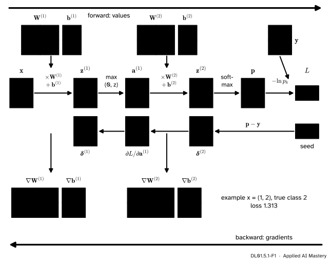
The running network of this module on its one example. Forward values (vermillion) fill the nodes from left to right. Gradients (green) come back from the loss, and each parameter collects its own.
Read the picture from right to left. The loss is 1.313 because the network gave the true class only 0.269. The gradient at the logits says: lower the first logit, raise the second. Each layer then passes that message back in the only way it can. A weight matrix passes it through its transpose; a ReLU passes it where the unit was on and blocks it where it was off; a bias simply receives a copy. That is backpropagation, the reverse mode of M05.9.1 run on a network with two outputs, a softmax and ReLUs.
Build it up
Step 1. The network, fixed for the course. Two inputs, two ReLU hidden units, two output classes. With the notation of the course, \(D = 2\) layers:
\(\vect{z}^{(2)}\) holds the logits, and \(k\) is the true class. The weights, used again by the module’s interactive, by DL01.6.4 and by DL01.7.2, are
The example is \({\vect{x}} = {(1, 2)}\) with true class 2, so the one-hot target is \({\vect{y}} = {(0, 1)}\).
Step 2. Forward, recording everything.\({\mat{W}^{(1)}\vect{x}} = {(1 - 1,\; -0.5 + 2)} = {(0, 1.5)}\), and adding the bias gives \({\vect{z}^{(1)}} = {(0.5, 1)}\). Both entries are positive, so the ReLU keeps them: \({\vect{a}^{(1)}} = {(0.5, 1)}\). Then \({\mat{W}^{(2)}\vect{a}^{(1)}} = {(0.5 + 1,\; -0.5 + 0.5)} = {(1.5, 0)}\) and the logits are \({\vect{z}^{(2)}} = {(1, 0)}\). The softmax gives \({p_1} = {e/(e + 1)} \approx {0.731}\) and \({p_2} \approx {0.269}\), and the loss is \({-\ln 0.269} \approx {1.313}\).
Step 3. Start at the logits. For softmax followed by cross-entropy the two local derivatives combine into one clean rule, derived below:
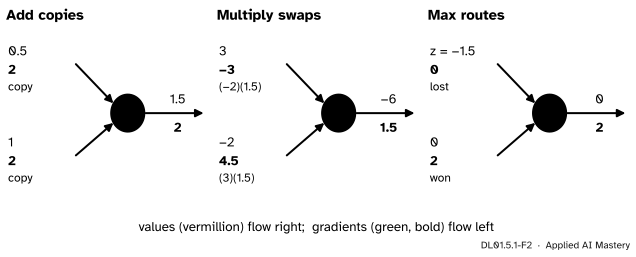
Step 4. Three patterns. Every operation in the network is built from additions, multiplications and one maximum, and each of these passes a gradient back in a fixed way.
DL01.5.1-F2
The three patterns of backward flow. An add node copies the gradient to each input. A multiply node gives each input the gradient times the other input. A max node sends the whole gradient to the input that won and nothing to the other: this is how a ReLU stops the gradient of a unit that is off.
Step 5. Through the output layer.\(\vect{z}^{(2)}\) is an addition, so \(\vect{b}^{(2)}\) gets a copy: \({\nabla_{\vect{b}^{(2)}}L} = {\vect{\delta}^{(2)}}\). The product \(\mat{W}^{(2)}\vect{a}^{(1)}\) is a multiplication, so the gradients swap: the weights get the gradient times the activations, \({\nabla_{\mat{W}^{(2)}}L} = {\vect{\delta}^{(2)}\vect{a}^{(1)\top}}\), and the activations get the gradient times the weights, \({\mat{W}^{(2)\top}\vect{\delta}^{(2)}} = {(1.462, 0.366)}\).
Step 6. Through the ReLU and the first layer. The ReLU is \({\max(0, z)}\), so it routes: both units were on, so both entries pass, and \({\vect{\delta}^{(1)}} = {(1.462, 0.366)}\). The first layer repeats Step 5: \({\nabla_{\vect{b}^{(1)}}L} = {\vect{\delta}^{(1)}}\) and \({\nabla_{\mat{W}^{(1)}}L} = {\vect{\delta}^{(1)}\vect{x}\T}\).
where \(z_j\) are the entries of \(\vect{z}^{(2)}\). Differentiate with respect to one logit \(z_i\). The first term gives \(-1\) if \({i} = {k}\) and 0 otherwise, which is \(-y_i\). The second term is the log of a sum, so its derivative is the derivative of the sum, \(e^{z_i}\), over the sum itself:
This is the result of M05.7.3, reached here without the softmax Jacobian.
DL01.5.1-F3
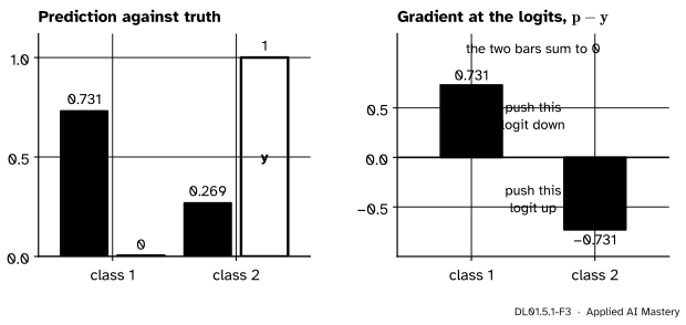
The gradient at the logits is the prediction minus the truth. It is positive for the class that got too much probability and negative for the true class, and its entries always sum to zero because both \(\vect{p}\) and \(\vect{y}\) sum to one.
A dense layer. Take \({\vect{z}} = {\mat{W}\vect{a} + \vect{b}}\), so \({z_i} = {\sum_j w_{ij}a_j + b_i}\). The weight \(w_{ij}\) appears once, multiplied by \(a_j\), so \({\partial z_i/\partial w_{ij}} = {a_j}\) and \({\partial L/\partial w_{ij}} = {\delta_i a_j}\), the entry \((i, j)\) of \({\vect{\delta}\vect{a}\T}\). The bias appears once with coefficient 1, so its gradient is \(\delta_i\). The input \(a_j\) appears in every\(z_i\), with coefficient \(w_{ij}\), so by the chain rule summed over those paths (M05.4.2)
The ReLU.\({a} = {\max(0, z)}\) has slope 1 for \({z > 0}\) and 0 for \({z < 0}\), so the gradient is multiplied by 1 or by 0: the mask. At exactly \({z} = {0}\) there is no slope; code picks a value there (DL01.3.2), and the running example stays clear of it. Prince’s summary of the backward pass, equation 7.25, is exactly this recurrence: multiply by the transposed weights, then by the indicator of the positive pre-activations.
Worked example
Every number, to three decimals, computed from unrounded values.
DL01.5.1-F4
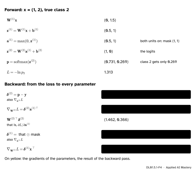
The worked trace. Each forward line uses only the line above it; each backward line uses the line above it and one value recorded on the way forward.
With \({e^1} \approx {2.718}\), \({p_1} = {2.718/3.718} \approx {0.731}\) and \({p_2} \approx {0.269}\).
Backward.
\({\vect{\delta}^{(2)}} = {(0.731 - 0,\; 0.269 - 1)} = {(0.731, -0.731)}\), which is also \({\nabla_{\vect{b}^{(2)}}L}\).
\({\nabla_{\mat{W}^{(2)}}L}\) has rows \({0.731 \times (0.5, 1)} = {(0.366, 0.731)}\) and \({-0.731 \times (0.5, 1)} = {(-0.366, -0.731)}\).
\({\mat{W}^{(2)\top}\vect{\delta}^{(2)}}\): the first column of \(\mat{W}^{(2)}\) is \({(1, -1)}\), giving \({0.731 + 0.731} = {1.462}\); the second is \({(1, 0.5)}\), giving \({0.731 - 0.366} = {0.366}\).
The mask is \({(1, 1)}\), so \({\vect{\delta}^{(1)}} = {(1.462, 0.366)}\), also \({\nabla_{\vect{b}^{(1)}}L}\).
\({\nabla_{\mat{W}^{(1)}}L}\) has rows \({1.462 \times (1, 2)} = {(1.462, 2.924)}\) and \({0.366 \times (1, 2)} = {(0.366, 0.731)}\).
What the numbers say. \({w^{(1)}_{12}}\) has the largest gradient, 2.924, because it multiplies the largest input, \({x_2} = {2}\), in the unit with the largest \(\delta\). A step of gradient descent lowers every weight with a positive gradient and raises those with a negative one, which pushes the first logit down and the second up, as the picture of the logits asked.
Code
From scratch: the forward pass with every value kept, then the backward pass as the six lines of the formal statement.
import numpy as npx, k = np.array([1.0, 2.0]), 1# class 2 is index 1 in codey = np.eye(2)[k]W1, b1 = np.array([[1.0, -0.5], [-0.5, 1.0]]), np.array([0.5, -0.5])W2, b2 = np.array([[1.0, 1.0], [-1.0, 0.5]]), np.array([-0.5, 0.0])def softmax(z): e = np.exp(z - z.max()) # shifting the logits leaves softmax unchangedreturn e / e.sum()z1 = W1 @ x + b1; a1 = np.maximum(z1, 0.0) # forward, values recordedz2 = W2 @ a1 + b2; p = softmax(z2)loss =-np.log(p[k])d2 = p - y # backwardgW2, gb2 = np.outer(d2, a1), d2ga1 = W2.T @ d2d1 = ga1 * (z1 >0) # the ReLU maskgW1, gb1 = np.outer(d1, x), d1print("p =", p.round(3), " loss =", round(loss, 3))print("grad W1 =", gW1.round(3).tolist(), " grad b1 =", gb1.round(3))print("grad W2 =", gW2.round(3).tolist(), " grad b2 =", gb2.round(3))
p = [0.731 0.269]  loss = 1.313
grad W1 = [[1.462, 2.924], [0.366, 0.731]]  grad b1 = [1.462 0.366]
grad W2 = [[0.366, 0.731], [-0.366, -0.731]]  grad b2 = [ 0.731 -0.731]
The independent check of M05.9.3: nudge each of the twelve parameters up and down by \({h} = {10^{-5}}\) and difference the loss.
def loss_of(params): w1, c1, w2, c2 = params q = softmax(w2 @ np.maximum(w1 @ x + c1, 0.0) + c2)return-np.log(q[k])params, grads, h = [W1, b1, W2, b2], [gW1, gb1, gW2, gb2], 1e-5worst =0.0for i, (P, G) inenumerate(zip(params, grads)):for idx in np.ndindex(P.shape): up = [q.copy() for q in params]; down = [q.copy() for q in params] up[i][idx] += h; down[i][idx] -= h numeric = (loss_of(up) - loss_of(down)) / (2* h) worst =max(worst, abs(numeric - G[idx]))print("largest gap between backprop and central differences:", f"{worst:.1e}")
largest gap between backprop and central differences: 9.2e-11
SciPy has the same check built in. scipy.optimize.check_grad takes the loss and the gradient as functions of one flat parameter vector and returns the length of their difference.
from scipy.optimize import check_graddef unflatten(theta):return [theta[:4].reshape(2, 2), theta[4:6], theta[6:10].reshape(2, 2), theta[10:]]def flat_grad(theta): w1, c1, w2, c2 = unflatten(theta) zz = w1 @ x + c1; aa = np.maximum(zz, 0.0) dd2 = softmax(w2 @ aa + c2) - y dd1 = (w2.T @ dd2) * (zz >0)return np.concatenate([np.outer(dd1, x).ravel(), dd1, np.outer(dd2, aa).ravel(), dd2])theta = np.concatenate([q.ravel() for q in params])print("check_grad:", f"{check_grad(lambda th: loss_of(unflatten(th)), flat_grad, theta):.1e}")
check_grad: 4.1e-08
The two agree to about the accuracy a finite difference can give. DL01.6.4 and DL01.7.2 will ask an engine of your own and then PyTorch to reproduce these twelve numbers.
Explore
DL01.5-X1
Backprop stepper
Press Step to fill in the forward pass node by node, then keep going for the backward pass; the read-out names the local rule used at each step. Then set the input to \({(-1, 1)}\) and watch hidden unit 1 switch off: its gradient stops at the ReLU and its weights get nothing.
Pitfalls
DL01.5.1-F5
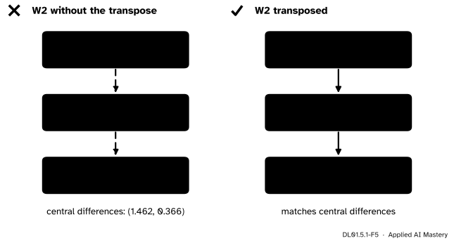
Wrong beside right. With a square weight matrix both products have the right shape, so the bug runs without an error. Only a gradient check shows that the left-hand numbers are wrong.
“The shapes match, so the backward pass is right.”
\(\mat{W}^{(2)}\) is 2 by 2, so \(\mat{W}^{(2)}\vect{\delta}^{(2)}\) and \(\mat{W}^{(2)\top}\vect{\delta}^{(2)}\) have the same shape. The first gives \({(0, -1.097)}\), the second the true \({(1.462, 0.366)}\). The transpose comes from summing over the output index \(i\) in \({\sum_i \delta_i w_{ij}}\). Square matrices hide this bug; a central-difference check catches it.
“The ReLU’s backward multiplies by its output.”
The local derivative of a ReLU is the mask, 1 or 0, not the activation. Multiplying by \({\vect{a}^{(1)}} = {(0.5, 1)}\) instead would give \({(0.731, 0.366)}\) in place of \({(1.462, 0.366)}\). For tanh the backward pass is written with the output, \({1 - a^2}\) (M05.9.1), which is where the habit comes from.
“The gradient with respect to the input is wasted work.”
It costs one more product, \({\mat{W}^{(1)\top}\vect{\delta}^{(1)}} \approx {(1.279, -0.366)}\), and it says how the loss changes as the input moves. Machine learning uses it to see which pixels a classifier relies on (a saliency map) and to build adversarial examples. In a deeper network, it is exactly the gradient that the layer below needs.
Check yourself
Recall
1. What is the gradient of the cross-entropy loss with respect to the logits when the output is a softmax?
Show answer
\({\vect{p} - \vect{y}}\): the predicted probabilities minus the one-hot target.
2. Name the three patterns of backward flow and what each does.
Show answer
An add node copies the gradient to every input. A multiply node gives each input the gradient times the other input. A max node sends the whole gradient to the input that won and 0 to the others.
3. For a dense layer \({\vect{z}} = {\mat{W}\vect{a} + \vect{b}}\) with gradient \(\vect{\delta}\) at \(\vect{z}\), what are the gradients of \(\mat{W}\), \(\vect{b}\) and \(\vect{a}\)?
Show answer
\({\vect{\delta}\vect{a}\T}\), \(\vect{\delta}\), and \({\mat{W}\T\vect{\delta}}\).
4. How does a gradient pass back through a ReLU?
Show answer
It is multiplied entry by entry by the mask \({\mathbb{I}[\vect{z} > 0]}\): it passes where the unit was on and stops where it was off.
5. Why does \({w^{(1)}_{12}}\) get the largest gradient in the worked example?
Show answer
Its gradient is \({\delta^{(1)}_1 x_2}\), the product of the largest hidden gradient, 1.462, and the largest input, 2.
Exercises
1.★ Run both passes by hand for the second example of the module, \({\vect{x}} = {(-1, 1)}\) with true class 1. Which gradients are zero, and why?
Show solution
Forward: \({\mat{W}^{(1)}\vect{x}} = {(-1 - 0.5,\; 0.5 + 1)} = {(-1.5, 1.5)}\), so \({\vect{z}^{(1)}} = {(-1, 1)}\), the mask is \({(0, 1)}\) and \({\vect{a}^{(1)}} = {(0, 1)}\). The logits are \({(0 + 1 - 0.5,\; 0 + 0.5 + 0)} = {(0.5, 0.5)}\), so \({\vect{p}} = {(0.5, 0.5)}\) and \({L} = {\ln 2} \approx {0.693}\).
Backward: \({\vect{\delta}^{(2)}} = {(0.5 - 1,\; 0.5 - 0)} = {(-0.5, 0.5)}\), the gradient of \(\vect{b}^{(2)}\). \({\nabla_{\mat{W}^{(2)}}L}\) has rows \({-0.5 \times (0, 1)} = {(0, -0.5)}\) and \({(0, 0.5)}\). \({\mat{W}^{(2)\top}\vect{\delta}^{(2)}} = {(-0.5 - 0.5,\; -0.5 + 0.25)} = {(-1, -0.25)}\), and the mask turns it into \({\vect{\delta}^{(1)}} = {(0, -0.25)}\). So \({\nabla_{\mat{W}^{(1)}}L}\) has rows \({(0, 0)}\) and \({-0.25 \times (-1, 1)} = {(0.25, -0.25)}\).
Zero: the first column of \({\nabla_{\mat{W}^{(2)}}L}\), because \({a^{(1)}_1} = {0}\) multiplies it; and the whole first row of \({\nabla_{\mat{W}^{(1)}}L}\) with \({\partial L/\partial b^{(1)}_1}\), because hidden unit 1 is off and the max node routed its gradient of \(-1\) to the constant 0.
2.★★ Show that for two classes \({p_1} = {\sigma(z_1 - z_2)}\), where \(\sigma\) is the sigmoid, and that the gradient at the logits is always \({(p_1 - y_1)\,(1, -1)}\).
Show solution
Divide the top and bottom of \({p_1} = {e^{z_1}/(e^{z_1} + e^{z_2})}\) by \(e^{z_1}\): \({p_1} = {1/(1 + e^{-(z_1 - z_2)})}\), which is \({\sigma(z_1 - z_2)}\). For the gradient, \({\vect{\delta}^{(2)}} = {(p_1 - y_1,\; p_2 - y_2)}\). Both \(\vect{p}\) and \(\vect{y}\) sum to 1, so \({p_2 - y_2} = {(1 - p_1) - (1 - y_1)} = {-(p_1 - y_1)}\). Hence \({\vect{\delta}^{(2)}} = {(p_1 - y_1)(1, -1)}\). In the worked example \({p_1 - y_1} = {0.731}\).
3.★★★ Keep \({\vect{x}} = {(1, 2)}\) but change the true class to 1. Without redoing the backward pass, explain why every one of the twelve gradients is the old one times the same number, and find that number.
Show solution
The forward pass does not depend on the label, so \(\vect{z}^{(1)}\), the mask, \(\vect{a}^{(1)}\) and \(\vect{p}\) are unchanged. By Exercise 2 the new gradient at the logits is \({(p_1 - 1)(1, -1)} = {-0.269\,(1, -1)}\), while the old one was \({0.731\,(1, -1)}\). Every later step of the backward pass is linear in the gradient it receives (products with fixed matrices, a fixed mask, outer products with fixed vectors), so every gradient is scaled by the same factor \({(p_1 - 1)/p_1} = {-0.269/0.731} \approx {-0.368}\). For instance \({\partial L/\partial w^{(1)}_{12}}\) becomes \({2.924 \times (-0.368)} \approx {-1.076}\).
Summary card
Backpropagation is the chain rule, one node at a time, from the loss back.
DL01.5.1-F1
Values forward, gradients back.
Logits: \({\vect{\delta}^{(2)}} = {\vect{p} - \vect{y}}\) for softmax with cross-entropy.
ReLU: times the mask \({\mathbb{I}[\vect{z} > 0]}\).
Add copies, multiply swaps, max routes.
Sources and next steps
Sources. Each was opened and checked against this lesson on 15 November 2026.
Stanford CS231n, Backpropagation, Intuitions. The section “Patterns in backward flow”: the add gate distributes the gradient equally to all its inputs, the max gate sends it unchanged to exactly one input, and the multiply gate’s local gradients are the input values, switched. The section on vectorised operations derives dW = dD.dot(X.T) and dX = W.T.dot(dD) by dimension analysis.
S. J. D. Prince, Understanding Deep Learning (MIT Press, 2023), section 7.4: the backward pass alternately multiplies by the transposed weight matrices and thresholds with the indicator \({\mathbb{I}[\vect{f}_{k-1} > 0]}\), summarised in equation 7.25; the weight gradient is the outer product of equation 7.23.
I. Goodfellow, Y. Bengio and A. Courville, Deep Learning (MIT Press, 2016). Algorithm 6.4 (section 6.5.4) is the backward computation for a deep network shown here; section 6.5.9 notes that the gradient of softmax with cross-entropy takes the simple form \({q_i - p_i}\) in its notation.