Put several neurons side by side on the same input and their weight vectors stack into the rows of a matrix. A layer computes phi(Wx + b) for one example and phi(XW^T + 1b^T) for a batch. Learn the shapes, count the parameters and read the outputs as new features.
DL01.1.3L2 Intermediate25 minIn review (what this means)
The maths and code on this page are checked by automated tests on every change, but an independent reader has not signed it off yet. Spot a mistake or a confusing step? Tell us.
Stack the weight vectors of several neurons into a weight matrix, and compute a layer’s output for one example.
Compute a layer on a batch with rows as examples, and state the shape of every array.
Count the parameters of a layer as n_out (n_in + 1).
Read the outputs of a layer as new features of the data, and test whether a classifier can use them.
The question
The digit classifier at the end of this course reads 64 pixels and passes them to 32 neurons at once. Writing out 32 weighted sums of 64 terms each, for every image, would be hopeless by hand and slow in a Python loop. How do 32 neurons become one operation on a whole batch of images, and how many numbers do they learn?
From the last lesson
1. Write the perceptron’s update rule for \(\vect{w}\) and \(b\).
Show answer
\({\vect{w} \leftarrow \vect{w} + \eta(y - \hat{y})\vect{x}}\) and \({b \leftarrow b + \eta(y - \hat{y})}\).
2. What happens when the perceptron is run on XOR?
Show answer
It never settles: it makes mistakes in every epoch and cycles through the same weights.
Intuition
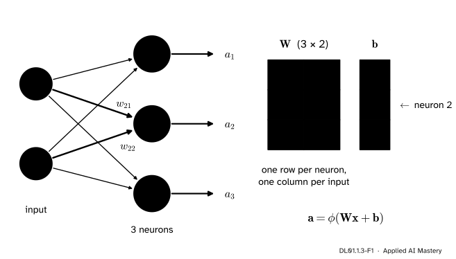
Take several neurons and give them all the same input. Each has its own weights and its own bias, so each computes its own weighted sum and its own output. Side by side they form a layer.
DL01.1.3-F1
A layer of three neurons on two inputs. The weights of neuron \(i\) fill row \(i\) of the weight matrix\(\mat{W}\), and its bias is entry \(i\) of \(\vect{b}\). Neuron 2 is picked out in both views.
The picture on the right is the whole lesson. Each neuron is a row of \(\mat{W}\). The product \(\mat{W}\vect{x}\) takes the dot product of each row with \(\vect{x}\), so it computes every neuron’s weighted sum at once. Add the bias vector, apply the activation to every entry, and the layer is done.
Build it up
Step 1. Three neurons, written out. With inputs \(\vect{x} = (x_1, x_2)\), three neurons compute
Row \(i\) of \({\mat{W}\vect{x}}\) is the dot product of row \(i\) of \(\mat{W}\) with \(\vect{x}\) (M02.5), which is neuron \(i\)’s weighted sum without its bias. So the three lines of Step 1 are one line: \({\vect{z} = \mat{W}\vect{x} + \vect{b}}\).
Step 3. Activate entry by entry. The activation acts on each entry on its own: \({\vect{a} = \phi(\vect{z}) = (\phi(z_1), \phi(z_2), \phi(z_3))}\). The outputs \(\vect{a}\) are called the layer’s activations.
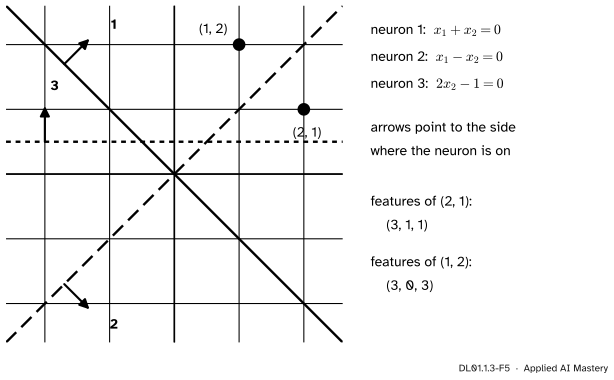
Step 4. Each neuron draws a line. Each row of \(\mat{W}\), with its bias, defines a line \({z_i = 0}\) in the input plane, exactly as the perceptron did. A layer of three neurons cuts the plane with three lines. With the ReLU, a point’s activation from a neuron is 0 on that neuron’s off side and grows with the distance beyond its line on the on side.
DL01.1.3-F5
The layer of the worked example seen in the input plane. Each neuron has its own line, and its weight vector points to the side where its weighted sum is positive. The point \((1, 2)\) is on the off side of neuron 2, so its second feature is 0.
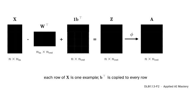
Step 5. A batch. In practice a layer processes many examples at once. Stack them as the rows of a matrix \(\mat{X}\), one row per example, which is how data tables and NumPy arrays are laid out. The next section shows that the whole batch is then one matrix product.
DL01.1.3-F2
The shapes of a layer on a batch of \({n = 4}\) examples with \({n_{\text{in}} = 2}\) inputs and \({n_{\text{out}} = 3}\) neurons. The bias row is copied to every example.
The formal statement
NoteDefinition: a fully connected layer
A layer with \(n_{\text{in}}\) inputs and \(n_{\text{out}}\) neurons has a weight matrix \(\cparam{\mat{W}}\) of shape \({n_{\text{out}} \times n_{\text{in}}}\), a bias vector \(\cparam{\vect{b}}\) of length \(n_{\text{out}}\) and an activation \(\phi\) applied entry by entry. For one input \(\cdata{\vect{x}}\),
where \(\vect{1}\) is a column of \(n\) ones, so that \({\vect{1}\vect{b}\T}\) repeats \(\vect{b}\T\) in every row.
Why the batch formula has a transpose. Row \(i\) of \(\mat{X}\) is \(\vect{x}_i\T\), and the layer’s weighted sums for that example are the column \({\mat{W}\vect{x}_i + \vect{b}}\). To store them as row \(i\) of \(\mat{Z}\), transpose, using \({(\mat{A}\mat{B})\T = \mat{B}\T\mat{A}\T}\):
Stacking these rows for \({i = 1, \dots, n}\) stacks the \(\vect{x}_i\T\) into \(\mat{X}\), and gives \({\mat{Z} = \mat{X}\mat{W}\T + \vect{1}\vect{b}\T}\). In NumPy the term \({\vect{1}\vect{b}\T}\) is written + b: broadcasting copies the vector to every row.
The shapes.
Array
Shape
Holds
\(\mat{X}\)
\({n \times n_{\text{in}}}\)
one example per row
\(\mat{W}\)
\({n_{\text{out}} \times n_{\text{in}}}\)
one neuron per row
\(\vect{b}\)
\(n_{\text{out}}\)
one bias per neuron
\(\mat{Z}\), \(\mat{A}\)
\({n \times n_{\text{out}}}\)
one example per row
\(\mat{W}\) keeps the shape (out, in), the shape in which PyTorch’s nn.Linear stores its weight (DL01.7.3). M05.7.3, and scikit-learn’s MLPClassifier (DL01.2.2), write a layer as \(\mat{X}\mat{W}\) with \(\mat{W}\) of shape (in, out): the same layer, with the matrix stored transposed.
Counting parameters. Each neuron has \(n_{\text{in}}\) weights and one bias, so a layer has
parameters. The digit network’s hidden layer has \({32 \cdot (64 + 1) = 2{,}080}\); its output layer, ten neurons on 32 inputs, has \({10 \cdot 33 = 330}\); together \({2{,}410}\), the number that DL01.7.3 checks in PyTorch.
Outputs as features. A layer replaces each example’s \(n_{\text{in}}\) numbers by \(n_{\text{out}}\) new ones. Any model placed after the layer sees only these new numbers, so the layer decides which features of the data the rest of the network can use. With fixed random weights it is a random feature map; once the weights are trained (DL01.2 onwards), the network chooses its own features.
Worked example
A layer of three ReLU neurons on a batch of two examples. Take
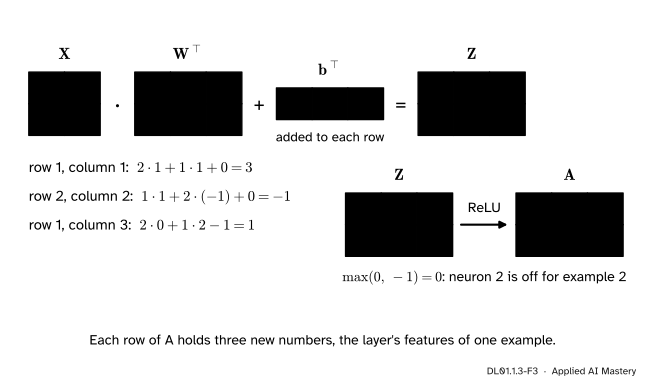
The batch holds the examples \((2, 1)\) and \((1, 2)\). Each entry of \({\mat{X}\mat{W}\T}\) is an example (a row of \(\mat{X}\)) dotted with a neuron (a row of \(\mat{W}\)). For the first example:
neuron 1: \({2 \cdot 1 + 1 \cdot 1 + 0 = 3}\);
neuron 2: \({2 \cdot 1 + 1 \cdot (-1) + 0 = 1}\);
neuron 3: \({2 \cdot 0 + 1 \cdot 2 - 1 = 1}\).
For the second: \({1 + 2 = 3}\), \({1 - 2 = -1}\) and \({0 + 4 - 1 = 3}\). So
The worked example as a trace. Every entry of \(\mat{Z}\) is one example dotted with one neuron, plus that neuron’s bias; ReLU then zeroes the single negative entry.
Read the rows of \(\mat{A}\) as features. The example \((2, 1)\) is described by \((3, 1, 1)\) and \((1, 2)\) by \((3, 0, 3)\): neuron 1 gives both the same value, neuron 2 is on for one and off for the other, and neuron 3 tells them apart by how high they sit. The layer has \({3 \cdot (2 + 1) = 9}\) parameters.
Code
A layer as a NumPy function, with every shape asserted, so that a transposed matrix fails loudly instead of computing the wrong thing.
import numpy as npdef relu(z):return np.maximum(z, 0.0)def layer(X, W, b, phi):"""A fully connected layer on a batch. X is (n, n_in), W is (n_out, n_in), b is (n_out,).""" n, n_in = X.shapeassert b.ndim ==1, f"b must be a vector of length n_out, got shape {b.shape}" n_out = b.shape[0]assert W.shape == (n_out, n_in), f"W must be (n_out, n_in) = ({n_out}, {n_in}), got {W.shape}" Z = X @ W.T + b # broadcasting adds b to every row: the 1 b^T of the formulaassert Z.shape == (n, n_out)return phi(Z)def n_params(n_in, n_out):return n_out * (n_in +1)W = np.array([[1.0, 1.0], [1.0, -1.0], [0.0, 2.0]])b = np.array([0.0, 0.0, -1.0])X = np.array([[2.0, 1.0], [1.0, 2.0]])A = layer(X, W, b, relu)print(A)print("parameters:", n_params(2, 3), " digit network:", n_params(64, 32) + n_params(32, 10))
The batch formula agrees with three neurons computed one at a time in a loop, and the shape checks catch the classic slip of multiplying by \(\mat{W}\) instead of \(\mat{W}\T\).
loop = np.array([[relu(W[i] @ x + b[i]) for i inrange(3)] for x in X])print("loop equals batch:", np.array_equal(loop, A))try: layer(X, W.T, b, relu) # W stored as (in, out) by mistakeexceptAssertionErroras error:print("caught:", error)
loop equals batch: True
caught: W must be (n_out, n_in) = (3, 2), got (2, 3)
Now the outputs as features. Take the two moons of scikit-learn (200 points, the course’s running two-class set) and a layer of 50 ReLU neurons with random weights that are never trained. A logistic regression on the raw two coordinates can only draw a straight boundary; the same model on the 50 features of the layer does much better.
from sklearn.datasets import make_moonsfrom sklearn.linear_model import LogisticRegressionX_moons, y_moons = make_moons(n_samples=200, noise=0.2, random_state=0)rng = np.random.default_rng(0)W_rand = rng.normal(size=(50, 2))b_rand = rng.normal(size=50)F = layer(X_moons, W_rand, b_rand, relu) # (200, 2) in, (200, 50) outraw = LogisticRegression().fit(X_moons, y_moons).score(X_moons, y_moons)feat = LogisticRegression().fit(F, y_moons).score(F, y_moons)print("feature array:", F.shape, " layer parameters:", n_params(2, 50))print(f"training accuracy on the raw inputs: {raw:.3f} on the layer's features: {feat:.3f}")
feature array: (200, 50)  layer parameters: 150
training accuracy on the raw inputs: 0.840   on the layer's features: 0.945
The accuracies are on the training points (with scikit-learn’s default penalty, C=1), so they measure what each set of features can express, not how well it generalises; ML01.2 explains the difference. The point is the jump from about 84 to about 94 percent without training the layer at all: new features made a linear model stronger. Choosing those features well is what training a network does.
Explore
The module’s interactive is in lesson 2. It shows one neuron, one row of \(\mat{W}\): each setting of its sliders is one line of the picture in Step 4.
Pitfalls
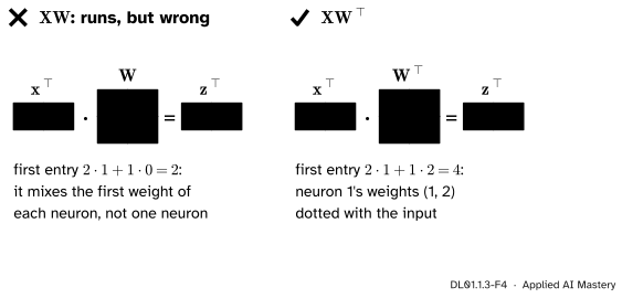
DL01.1.3-F4
Wrong beside right, for a layer with neurons \((1, 2)\) and \((0, 1)\) on the input \((2, 1)\). With a square \(\mat{W}\) both products run, and only one is the layer.
“If the matrix product runs, the shapes are right.”
When \({n_{\text{in}} = n_{\text{out}}}\), \(\mat{W}\) is square and \(\mat{X}\mat{W}\) runs just as happily as \(\mat{X}\mat{W}\T\). It dots each example with the columns of \(\mat{W}\), which mix the weights of different neurons. Write the shapes down, or assert them, as the layer function does.
“The bias is added once to the whole batch.”
It is added to every row: each example gets every neuron’s bias. In NumPy, X @ W.T + b with b of shape (n_out,) does this. Writing b[:, None] instead, a column, broadcasts along the wrong axis; when \({n = n_{\text{out}}}\) it runs silently and adds bias \(i\) to example \(i\).
“A layer of several neurons draws a curved boundary.”
Each neuron still draws one straight line. A layer only produces features; a boundary appears when something reads them, such as another neuron. Lesson 4 shows that without an activation between them, even that does not bend the boundary.
Check yourself
Recall
1. In the weight matrix of a layer, what does row \(i\) hold, and what does column \(j\) hold?
Show answer
Row \(i\) holds the weights of neuron \(i\); column \(j\) holds every neuron’s weight on input \(j\).
2. Write a layer’s output for one example and for a batch with rows as examples.
3. What are the shapes of \(\mat{X}\), \(\mat{W}\) and \(\mat{Z}\) for a batch of \(n\) examples?
Show answer
\({n \times n_{\text{in}}}\), \({n_{\text{out}} \times n_{\text{in}}}\) and \({n \times n_{\text{out}}}\).
4. How many parameters does a layer with \(n_{\text{in}}\) inputs and \(n_{\text{out}}\) neurons have?
Show answer
\({n_{\text{out}}(n_{\text{in}} + 1)}\): a weight per neuron per input, plus a bias per neuron.
5. In the moons experiment, what changed between the 84 and the 94 percent accuracy?
Show answer
Only the inputs of the logistic regression: the raw two coordinates, or the 50 features of an untrained random ReLU layer.
Exercises
1.★ A network reads \(28 \times 28 = 784\) pixels into a layer of 128 neurons, then a layer of 10. How many parameters does each layer have, and how many in all?
Show solution
\({128 \cdot (784 + 1) = 100{,}480}\) and \({10 \cdot (128 + 1) = 1{,}290}\), so \({101{,}770}\) in all.
2.★★ For the layer of the worked example, compute the activations of the inputs \((-1, 1)\) and \((0, 0)\). What is the shape of \(\mat{Z}\) for a batch of 5 examples?
so \({\vect{a} = (0, 0, 1)}\). For \((0, 0)\): \({\vect{z} = \vect{b} = (0, 0, -1)}\), so \({\vect{a} = (0, 0, 0)}\). For 5 examples, \(\mat{Z}\) is \({5 \times 3}\).
3.★★★ Show that \({\mat{X}\mat{W}\T + \vect{1}\vect{b}\T = \tilde{\mat{X}}\tilde{\mat{W}}\T}\), where \(\tilde{\mat{X}}\) is \(\mat{X}\) with a column of ones appended and \(\tilde{\mat{W}}\) is \(\mat{W}\) with \(\vect{b}\) appended as a last column. Which lesson used the same trick?
Show solution
Write \({\tilde{\mat{X}} = [\,\mat{X} \;\; \vect{1}\,]}\) and \({\tilde{\mat{W}} = [\,\mat{W} \;\; \vect{b}\,]}\), so \({\tilde{\mat{W}}\T}\) stacks \(\mat{W}\T\) on top of the row \(\vect{b}\T\). Multiplying blocks,
Lesson 2 used the same trick for one neuron, folding the bias into the weights as \({\vect{\theta} = (\vect{w}, b)}\) with inputs \({\tilde{\vect{x}} = (\vect{x}, 1)}\).
Summary card
A layer is many neurons on one input: their weights are the rows of W.
DL01.1.3-F1
One row per neuron.
One example.\({\vect{a} = \phi(\mat{W}\vect{x} + \vect{b})}\), with \(\mat{W}\) of shape (out, in).
A batch.\({\mat{A} = \phi(\mat{X}\mat{W}\T + \vect{1}\vect{b}\T)}\), one example per row.
Parameters.\({n_{\text{out}}(n_{\text{in}} + 1)}\); the digit network has \({2{,}080 + 330 = 2{,}410}\).
Features. The rows of \(\mat{A}\) are new features of the examples.
Sources and next steps
Sources. Each was opened and checked against this lesson on 15 November 2026.
Stanford CS231n, Neural Networks Part 1: Setting up the Architecture, sections “Layer-wise organization” and “Example feed-forward computation”: “The forward pass of a fully-connected layer corresponds to one matrix multiplication followed by a bias offset”, and a network with layers of 4 and 2 neurons on 3 inputs has \({[3 \times 4] + [4 \times 2] = 20}\) weights and \({4 + 2 = 6}\) biases, 26 parameters in all.
Simon J. D. Prince, Understanding Deep Learning (MIT Press, 2023), Section 4.4, “Matrix notation”: a layer as an activation applied to a bias vector plus a weight matrix times the previous layer, with the weight matrix of size (units out) by (units in).
PyTorch 2.15 documentation, torch.nn.Linear: computes \({y = xA\T + b}\), with the weight of shape (out_features, in_features) and the bias of shape (out_features).
Next.DL01.1.4 What one layer cannot do asks whether a single layer, or a stack of layers with nothing between them, can classify XOR.