For K classes the network outputs K logits and the softmax turns them into a categorical distribution. The negative log-likelihood of the true class is minus its logit plus log-sum-exp, computed safely by subtracting the largest logit first. Its gradient is p - y.
DL01.4.3L2 Intermediate25 minIn review (what this means)
The maths and code on this page are checked by automated tests on every change, but an independent reader has not signed it off yet. Spot a mistake or a confusing step? Tell us.
Derive categorical cross-entropy for an integer label k as minus the logit z_k plus the log-sum-exp of the logits.
Prove that the softmax is unchanged when the same constant is added to every logit, and use it to compute log-sum-exp without overflow.
Recall and check the gradient p - y of cross-entropy with respect to the logits.
Split cross-entropy into an entropy and a Kullback-Leibler divergence, and compute both for a small example.
The question
A digit classifier has ten outputs, one per digit. Early in training one image gets the logits 1002, 1001 and 1000 for its three most likely classes. Compute the softmax as written, \(e^{z_k}\) over the sum of the \(e^{z_j}\), and every exponential overflows to infinity: the probabilities come out as nan. Yet the answer is perfectly ordinary. How is the loss for many classes built, and why does subtracting one number make it safe?
From the last lesson
1. Write binary cross-entropy as one formula in the logit \(z\) and the label \(y\).
2. What is its gradient with respect to the logit?
Show answer
\({p - y}\), where \({p = \sigma(z)}\).
Intuition
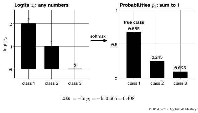
Two classes needed a coin; \(K\) classes need a die with \(K\) faces, each with its own probability. The network outputs one logit per class, any real numbers. The softmax turns them into probabilities: it exponentiates each logit, which makes it positive, and divides by the total, which makes them sum to 1. The loss is the surprise again, minus the log of the probability given to the class that was true.
DL01.4.3-F1
The logits \({\vect{z} = (2, 1, 0)}\) become the probabilities \({(0.665, 0.245, 0.090)}\). The true class is class 1, so the loss is \({-\ln 0.665 = 0.408}\).
Only the differences between logits matter: class 1 beats class 2 by one unit of logit, so it gets \(e\) times the probability. Add 1000 to every logit and none of the differences change, so the probabilities do not either. That observation is the whole of the numerical trick.
Build it up
Step 1. The categorical distribution. A label \(k\) in \({\{1, \dots, K\}}\) has probability \({P(y = k) = p_k}\), with every \({p_k \ge 0}\) and \({\sum_k p_k = 1}\).
Step 2. The softmax. From logits \({\vect{z} \in \R^K}\),
For \({\vect{z} = (2, 1, 0)}\) the exponentials are \({7.389, 2.718, 1}\), their sum is \({11.107}\), and the probabilities are \({(0.665, 0.245, 0.090)}\).
Step 3. Minus the log of the true class. For a true label \(k\), the log of a quotient is a difference of logs, and the log undoes the exponential on top:
For the example, \(\ell = -2 + {\ln 11.107} = -2 + 2.408 = 0.408\). This is categorical cross-entropy. The loss never needs \(p_k\) itself, only the logits.
Step 4. Adding a constant changes nothing. Add \(c\) to every logit:
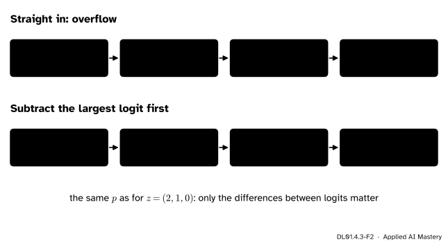
The factor \(e^{c}\) cancels. So \({(1002, 1001, 1000)}\) and \({(2, 1, 0)}\) give the same probabilities, although \({e^{1002}}\) is far beyond the largest 64-bit number, about \({1.8 \times 10^{308}}\).
DL01.4.3-F2
Subtracting the largest logit before exponentiating leaves the softmax unchanged and keeps every exponential between 0 and 1.
Step 5. The log-sum-exp trick. Let \({m = \max_j z_j}\). Take \(e^{m}\) out of the sum:
Every \({z_j - m \le 0}\), so no exponential overflows, and the largest term is \({e^{0} = 1}\), so the sum is at least 1 and its log is never \({\ln 0}\).
The formal statement
NoteCategorical cross-entropy
For logits \({\cmodel{\vect{z}} \in \R^K}\) and a true class \(k\) with one-hot target \(\ctruth{\vect{y}}\),
with \({m = \max_j z_j}\) and \({\vect{p} = \mathrm{softmax}(\vect{z})}\).
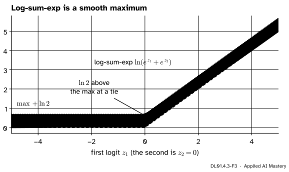
Log-sum-exp is a smooth maximum. The sum \({\sum_j e^{z_j - m}}\) has \(K\) terms, each at most 1, and one of them is \({e^0 = 1}\), so the sum lies between 1 and \(K\). Taking logs,
For two logits, log-sum-exp is a rounded version of the maximum. It is \({\ln 2}\) above the maximum at a tie and almost equal to it when one logit dominates.
So the loss \({-z_k + \mathrm{LSE}(\vect{z})}\) is roughly “the best logit minus the true one”. When the true class already has the largest logit by a wide margin, the loss is near 0. When another class wins by a margin \(d\), the loss is about \(d\): it grows like a straight line, just as the binary loss did.
The gradient, recalled from M05.7.3. The derivative of the log-sum-exp is the softmax: \({\partial\,\mathrm{LSE}/\partial z_j = e^{z_j}/\sum_i e^{z_i} = p_j}\). The derivative of \({-z_k}\) is \({-1}\) for \({j = k}\) and 0 otherwise, which is \({-y_j}\) for the one-hot \(\vect{y}\). Together, \({\partial\ell/\partial z_j = p_j - y_j}\). With \({K = 2}\) and logits \({(z, 0)}\) the softmax gives \({p_1 = e^{z}/(e^{z} + 1) = \sigma(z)}\), and everything reduces to the binary lesson.
Cross-entropy, entropy and divergence. For any target distribution \(\vect{y}\), not only a one-hot one, the cross-entropy is \({H(\vect{y}, \vect{p}) = -\sum_j y_j \ln p_j}\). Adding and subtracting \({\sum_j y_j \ln y_j}\) splits it in one line:
The entropy\({H(\vect{y})}\) does not depend on the network, so minimising cross-entropy minimises the Kullback-Leibler divergence of \(\vect{p}\) from \(\vect{y}\). For a one-hot target \({H(\vect{y}) = 0}\) (with \({0 \ln 0 = 0}\)) and the two are equal. KL in full is M09.3.
Worked example
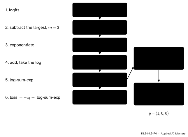
Logits \({\vect{z} = (2, 1, 0)}\), true class 1.
Largest logit \({m = 2}\); shifted logits \({(0, -1, -2)}\).
Exponentials \({(1, 0.3679, 0.1353)}\); their sum \({1.5032}\); its log \({0.4076}\).
Gradient descent lowers the logits of the wrong classes and raises the true one, and the three components of the gradient sum to 0, because \({\sum_j p_j = \sum_j y_j = 1}\).
DL01.4.3-F4
The stable computation, step by step, and the gradient it leads to.
A soft target. Suppose the target is not one-hot but \({\vect{y} = (0.7, 0.2, 0.1)}\), as when labels are smoothed. Then \({H(\vect{y}) = 0.802}\), \({H(\vect{y}, \vect{p}) = 0.808}\) and \({\mathrm{KL}(\vect{y} \,\|\, \vect{p}) = 0.006}\): the predicted distribution is already very close to this target.
Code
A stable log-softmax for a batch whose rows are examples, and the mean cross-entropy for integer labels (0, 1, 2 in code for classes 1, 2, 3).
import numpy as npdef log_softmax(Z): m = Z.max(axis=1, keepdims=True)return Z - m - np.log(np.exp(Z - m).sum(axis=1, keepdims=True))def cross_entropy(Z, labels):return-log_softmax(Z)[np.arange(len(labels)), labels].mean()z = np.array([[2.0, 1.0, 0.0]])p = np.exp(log_softmax(z))[0]print("p =", p.round(3), " loss =", round(cross_entropy(z, [0]), 4), " p - y =", (p - [1, 0, 0]).round(3))with np.errstate(over="ignore", invalid="ignore"): naive = np.exp(z +1000) / np.exp(z +1000).sum()print("naive softmax of z + 1000:", naive, " stable:", np.exp(log_softmax(z +1000))[0].round(3))
p = [0.665 0.245 0.09 ]  loss = 0.4076  p - y = [-0.335  0.245  0.09 ]
naive softmax of z + 1000: [[nan nan nan]]   stable: [0.665 0.245 0.09 ]
Now a small batch, checked against SciPy’s logsumexp and scikit-learn’s log_loss, and the split into entropy and divergence for the soft target:
The last row of the batch, three equal logits, has loss \({\ln 3 = 1.099}\): a model that has no preference among \(K\) classes always starts at \({\ln K}\).
Explore
The one-example loss explorer in lesson DL01.4.2 has a three-class mode. Choose Three classes (softmax), pick a true class, and slide its logit from far below the others to far above them: the cross-entropy follows the smooth maximum of this lesson, and its gradient \({p_k - 1}\) runs from \(-1\) to 0.
Pitfalls
DL01.4.3-F5
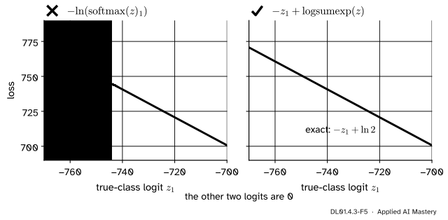
Wrong beside right. Taking the log of a softmax probability fails once that probability underflows to 0, below about \({z_1 = -745}\) here. The log-softmax \({z_1 - \mathrm{LSE}(\vect{z})}\) never forms the tiny probability.
“Compute the softmax, then take the log of the right entry.”
The probability of a badly wrong class can be smaller than the smallest positive 64-bit number, about \({5 \times 10^{-324}}\). It rounds to 0 and the loss becomes infinite (figure above). Even just above that limit the answer loses digits: at \({z_1 = -740}\) the naive loss is 740.702 where the true value is 740.693. Compute \({-z_k + \mathrm{LSE}(\vect{z})}\) directly.
“Apply a softmax, then hand the result to a loss that expects logits.”
Many library losses take logits and apply the log-softmax themselves (DL01.7.4). Feeding them probabilities applies the softmax twice. For \({\vect{z} = (2, 1, 0)}\) the second softmax turns \({(0.665, 0.245, 0.090)}\) into \({(0.451, 0.296, 0.253)}\), and the loss becomes 0.797 instead of 0.408. Worse, the result can never come near 1, so the loss never falls near 0 and the gradients stay small and misleading.
“Every label must be turned into a one-hot vector first.”
For a one-hot target the cross-entropy is just \({-\ln p_k}\), so the integer label \(k\) is enough: pick out one entry of the log-softmax. One-hot vectors, or soft ones, are only needed when the target puts probability on several classes.
Check yourself
Recall
1. Write categorical cross-entropy for logits \(\vect{z}\) and true class \(k\) in terms of the log-sum-exp.
Show answer
\({\ell = -z_k + \mathrm{LSE}(\vect{z})}\), with \({\mathrm{LSE}(\vect{z}) = \ln\sum_j e^{z_j}}\).
2. Why is the softmax unchanged when the same constant is added to every logit?
Show answer
Every exponential is multiplied by \(e^{c}\), top and bottom, and the factor cancels.
3. How is the log-sum-exp computed without overflow?
Show answer
Subtract the largest logit \(m\) first: \({\mathrm{LSE}(\vect{z}) = m + \ln\sum_j e^{z_j - m}}\). Every exponent is then at most 0, and the sum is at least 1.
4. What is the gradient of categorical cross-entropy with respect to the logits?
Show answer
\({\vect{p} - \vect{y}}\), the predicted probabilities minus the one-hot target.
5. How does cross-entropy split into an entropy and a divergence, and what happens for a one-hot target?
Show answer
\({H(\vect{y}, \vect{p}) = H(\vect{y}) + \mathrm{KL}(\vect{y} \,\|\, \vect{p})}\). For a one-hot target the entropy is 0, so cross-entropy equals the KL divergence.
Exercises
1.★ Logits \({(0, 0, 0, 0)}\) for four classes. Find the probabilities, the loss for any true class, and the gradient.
Show solution
All four probabilities are \({\tfrac14}\). The loss is \({-0 + \ln 4 = 1.386}\) whatever the true class. The gradient is \({\tfrac14}\) for each wrong class and \({\tfrac14 - 1 = -\tfrac34}\) for the true one.
2.★★ Compute the loss for logits \({(500, 0, -500)}\) with true class 2, using the log-sum-exp trick.
Show solution
\({m = 500}\), shifted logits \({(0, -500, -1000)}\). The sum \({1 + e^{-500} + e^{-1000}}\) is 1 to far more than 64-bit precision, so \({\mathrm{LSE} = 500 + \ln 1 = 500}\). The loss is \({-z_2 + 500 = 0 + 500 = 500}\): the true class lost to class 1 by a margin of 500, and the loss is that margin.
3.★★★ Show that for \({K = 2}\) and logits \({(z_1, z_2)}\), categorical cross-entropy with true class 1 equals binary cross-entropy with label 1 and logit \({z_1 - z_2}\).
Show solution
\(\ell = -z_1 + {\ln(e^{z_1} + e^{z_2})}\). Take \(e^{z_1}\) out of the bracket: \({\ln(e^{z_1} + e^{z_2})} = z_1 + {\ln(1 + e^{z_2 - z_1})}\). So \(\ell = {\ln(1 + e^{-(z_1 - z_2)})} = {\mathrm{softplus}(-(z_1 - z_2))}\), which is the binary loss of lesson 2 for \({y = 1}\) and logit \({z = z_1 - z_2}\). Only the difference of the two logits matters.
Summary card
Logits in, a die out; the loss is minus the log of the true face.
DL01.4.3-F1
Softmax, then the surprise of the true class.
Softmax:\({p_k = e^{z_k}/\sum_j e^{z_j}}\), unchanged by adding a constant to every logit.
Loss:\({\ell = -z_k + \mathrm{LSE}(\vect{z})}\), with \({\mathrm{LSE} = m + \ln\sum_j e^{z_j - m}}\).
Sources. Each was opened and checked against this lesson on 15 November 2026.
Simon J. D. Prince, Understanding Deep Learning, MIT Press, 2023 (free PDF). Section 5.5 builds the multiclass loss from the categorical distribution and the softmax (equations 5.21 to 5.24, with the loss as minus the true output plus the log of the sum of exponentials); Section 5.7 relates cross-entropy to the Kullback-Leibler divergence (equation 5.27 onwards).
Ian Goodfellow, Yoshua Bengio and Aaron Courville, Deep Learning, MIT Press, 2016. Section 6.2.2.3 writes the log-softmax as \({z_i - \log\sum_j \exp(z_j)}\) (equation 6.30), states that the softmax is invariant to adding the same scalar to all its inputs (6.32), and derives the stable form \({\mathrm{softmax}(\vect{z} - \max_i z_i)}\) (6.33).
SciPy documentation, scipy.special.logsumexp. The log of the sum of exponentials, computed in a numerically more stable way, with an axis argument.
scikit-learn 1.9 documentation, sklearn.metrics.log_loss. Accepts an array of class probabilities with one column per class, and a labels argument.