One training iteration in PyTorch is five lines: forward, loss, zero_grad, backward, step. See what each line reads and writes, why their order matters, and what goes wrong, with numbers, when a line is missing or out of place.
DL01.8.1L2 Intermediate25 minIn review (what this means)
The maths and code on this page are checked by automated tests on every change, but an independent reader has not signed it off yet. Spot a mistake or a confusing step? Tell us.
Write the five lines of one PyTorch training iteration in order and say what each one reads and writes.
Explain why backward adds into .grad, and compute what the buffer holds when zero_grad is left out.
Show that gradient descent without zero_grad oscillates for ever on a quadratic loss, whatever the learning rate.
Recognise the order bugs (no zero_grad, step before backward, backward twice) from their numbers.
The question
Every PyTorch training script, from a two-layer toy to a large language model, has the same five lines at its heart. Leave one out, or swap two, and the script still runs without a single error message, yet the network learns nothing or learns nonsense. What does each line actually do, and how can you tell from the numbers which one went wrong?
Intuition
Training is a loop, and one turn of the loop is one iteration: take a batch, measure how wrong the network is on it, and nudge every parameter to make it a little less wrong. In PyTorch that turn is five lines.
DL01.8.1-F1
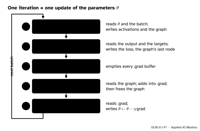
One iteration of training. Each line reads something and writes something, and the loop goes round once per batch. The colours follow the course: the forward pass is model, the loss is loss, gradients are grad and the parameters are param.
Think of the loop as four stores of numbers and five workers that take turns with them. The stores are the parameters\(\theta\) (every weight and bias), the activations together with the computational graph that records how they were computed, the gradient buffers (.grad, one per parameter) and the loss. The forward pass fills the activations and builds the graph. The loss adds the last node. zero_grad empties the buffers. backward walks the graph from the loss back to the parameters and adds each gradient into its buffer. step reads the buffers and moves the parameters.
Nothing in these lines checks that the others ran. That is why the bugs are silent: each worker does its job on whatever it finds in the stores.
Build it up
Step 1. The forward pass.out = model(X) reads the parameters and the batch. It writes the activations of every layer and, because the parameters have requires_grad=True, a graph of the operations that produced out (DL01.7.2). Nothing about the parameters changes.
Step 2. The loss.loss = loss_fn(out, y) compares the output with the targets and returns one number. It is the last node of the graph, so the graph now runs from the parameters all the way to the loss.
Step 3. Empty the buffers.optimizer.zero_grad() clears the .grad of every parameter the optimizer holds. By default (set_to_none=True) it sets each buffer to None rather than filling it with zeros, which saves memory. It touches nothing else.
Step 4. The backward pass.loss.backward() runs backpropagation through the graph, exactly the reverse sweep of DL01.5 and DL01.6. For each parameter it computes the partial derivative of the loss and adds it into .grad. Then it frees the graph, because the saved activations are no longer needed.
Step 5. The update.optimizer.step() reads every .grad and moves its parameter. For plain stochastic gradient descent that is \(\theta \leftarrow \theta - \eta\,\text{grad}\).
DL01.8.1-F2
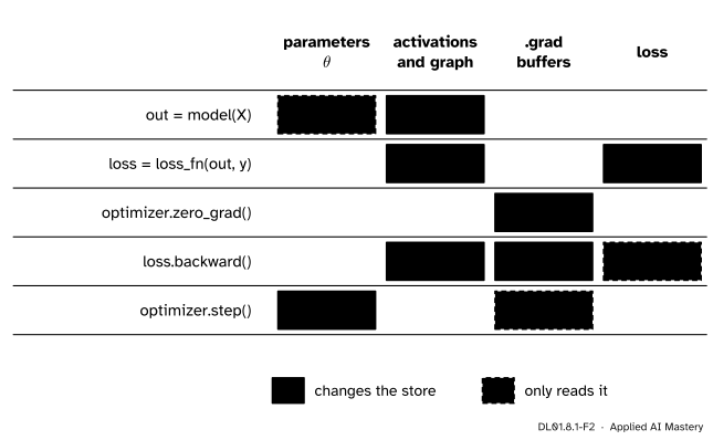
The same five lines as a table of reads and writes. Only step changes the parameters, and only backward and zero_grad change .grad.
Read the table down the .grad column. Two lines write it: zero_grad empties it and backward adds to it. So whatever step reads is the sum of every gradient added since the last zero_grad. The only requirement on order is therefore that zero_grad comes after the previous step and before this backward. Putting it first in the loop, as many scripts do, is equally correct.
The formal statement
NoteOne iteration of mini-batch gradient descent
Let \(L_t(\theta)\) be the mean loss on the batch drawn at iteration \(t\), and \(\vect{g}_t = \nabla L_t(\theta_t)\) its gradient at the current parameters. One iteration is
PyTorch splits it into five lines. backward performs \(\text{grad} \leftarrow \text{grad} + \vect{g}_t\), zero_grad resets the buffer, and step performs \(\theta \leftarrow \theta - \eta\, \text{grad}\).
With zero_grad in every iteration, the buffer holds exactly \(\vect{g}_t\) when step reads it, and the loop is the update above. This is the mini-batch gradient descent of ML01.5.4, now written by PyTorch.
Without zero_grad the buffer keeps everything. Write \(\vect{G}_t\) for what it holds at step \(t\):
Every past gradient keeps pushing, at full strength, for ever. To see where that leads, take the simplest loss with a minimum, a parabola along one direction: \({L(\theta) = \tfrac{h}{2}(\theta - \theta^\ast)^2}\) with curvature \(h > 0\). Its gradient is \({g_t = h e_t}\), where \({e_t = \theta_t - \theta^\ast}\) is the error at step \(t\).
Step 1: remove the sum. Write the update for two consecutive steps and subtract:
Step 4: read off the behaviour. If \({0 < \eta h < 4}\) the discriminant is negative, so the roots are a complex pair \(r\) and \(\bar r\) with \({r \bar r = \abs{r}^2 = 1}\). Both have size exactly 1, so the error is a cosine, \({e_t = A\cos(\omega t + \varphi)}\) with \({\cos\omega = 1 - \eta h/2}\), whose amplitude never shrinks. If \({\eta h > 4}\) the roots are real with product 1, so one of them is larger than 1 in size and the error grows. At \({\eta h = 4}\) the double root \(-1\) makes it grow linearly.
Compare the correct loop, where \({e_{t+1} = (1 - \eta h)\, e_t}\) shrinks for every \({0 < \eta h < 2}\) (ML01.5.3). Without zero_grad there is no learning rate at which the parameters settle.
DL01.8.1-F4
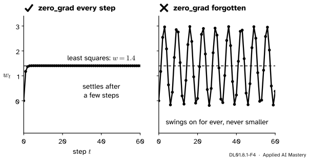
Gradient descent on the four points of ML01 from \({(w, b) = (0, 0)}\) with \({\eta = 0.05}\). With zero_grad the weight settles at the least-squares value 1.4. Without it the weight swings for ever.
The loss of the four points is a parabola in two directions, the eigenvectors of its Hessian \({\begin{bmatrix} 15 & 5 \\ 5 & 2 \end{bmatrix}}\), whose eigenvalues are about 16.70 and 0.299. With \({\eta = 0.05}\) the products \(\eta h\) are about 0.835 and 0.015, both between 0 and 4, so both directions swing: one with a period of about 6.6 steps (the fast wobble in the figure) and one with a period of about 51 steps.
Go deeper: accumulating on purpose
The adding is a feature. If a batch is too large for memory, split it into \(k\) micro-batches of equal size, call backward on each micro-batch loss divided by \(k\), and step once. Because the gradient of a sum is the sum of the gradients,
the buffer then holds the gradient of the mean loss of the whole batch, exactly as if it had been processed in one go. Exercise 3 checks this. Shared weights (DL01.5.3) rely on the same adding within a single backward pass. A buffer that adds up past gradients with a decay factor is momentum, the subject of DL02.1.
Worked example
Take the linear neuron of DL01.1.1 on the four points \({x = (1, 2, 3, 4)}\), \({y = (2, 3, 5, 6)}\) with the mean squared error, start at \({(w, b) = (0, 0)}\) and use \({\eta = 0.05}\). The gradient of the loss is
\[
\begin{aligned}
\pd{L}{w} &= \tfrac{2}{4}\textstyle\sum_i (w x_i + b - y_i)\, x_i, \\
\pd{L}{b} &= \tfrac{2}{4}\textstyle\sum_i (w x_i + b - y_i).
\end{aligned}
\]
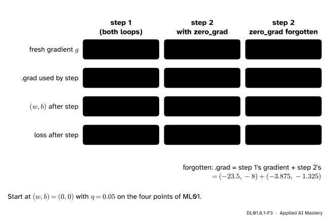
Step 1 (both loops). At \((0, 0)\) the residuals are \(-y\), so \({\pd{L}{w} = -\tfrac{2}{4} \cdot 47 = -23.5}\) and \({\pd{L}{b} = -\tfrac24 \cdot 16 = -8}\), as in ML01.5.2. The buffers start empty, so .grad holds \({(-23.5, -8)}\), and the step gives \({w = 0.05 \cdot 23.5 = 1.175}\) and \({b = 0.05 \cdot 8 = 0.4}\). The loss falls from 18.5 to about 0.552.
Step 2, fresh gradient. At \({(1.175, 0.4)}\) the predictions are 1.575, 2.75, 3.925 and 5.1, so the residuals are \(-0.425\), \(-0.25\), \(-1.075\) and \(-0.9\). Then
Step 2 with zero_grad. The buffer was emptied, so it holds \({(-3.875, -1.325)}\). The step gives \({w = 1.175 + 0.05 \cdot 3.875 = 1.36875}\) and \({b = 0.4 + 0.05 \cdot 1.325 = 0.46625}\), and the loss drops to about 0.0637.
Step 2 without zero_grad.backward adds the fresh gradient to what step 1 left behind:
The step is seven times too long: \({w = 1.175 + 0.05 \cdot 27.375 = 2.54375}\) and \({b = 0.4 + 0.05 \cdot 9.325 = 0.86625}\). The loss jumps from 0.552 to about 12.09.
DL01.8.1-F3
The worked example as a trace. The fresh gradient at step 2 is the same in both loops; only what .grad holds differs, and with it every number below.
Code
First the worked example in PyTorch. nn.Linear(1, 1) is the neuron, started at zero.
import numpy as npimport torchfrom torch import nntorch.set_num_threads(1)x = torch.tensor([[1.0], [2.0], [3.0], [4.0]])y = torch.tensor([[2.0], [3.0], [5.0], [6.0]])def neuron_run(steps, zero_grad=True, lr=0.05): model = nn.Linear(1, 1)with torch.no_grad(): # start at (w, b) = (0, 0) model.weight.zero_() model.bias.zero_() loss_fn = nn.MSELoss() optimizer = torch.optim.SGD(model.parameters(), lr=lr) rows = []for _ inrange(steps): out = model(x) # 1. forward loss = loss_fn(out, y) # 2. lossif zero_grad: optimizer.zero_grad() # 3. empty the buffers loss.backward() # 4. add gradients into .grad grad = (model.weight.grad.item(), model.bias.grad.item()) optimizer.step() # 5. update the parameters after = loss_fn(model(x), y).item() rows.append((grad, (model.weight.item(), model.bias.item()), after))return rowsfor name, flag in [("with zero_grad", True), ("forgotten", False)]:for k, (grad, wb, after) inenumerate(neuron_run(2, flag), 1):print(f"{name:15s} step {k}: .grad = ({grad[0]:8.3f}, {grad[1]:7.3f})"f" (w, b) = ({wb[0]:.5f}, {wb[1]:.5f}) loss = {after:.4f}")
with zero_grad  step 1: .grad = ( -23.500,  -8.000)  (w, b) = (1.17500, 0.40000)  loss = 0.5522
with zero_grad  step 2: .grad = (  -3.875,  -1.325)  (w, b) = (1.36875, 0.46625)  loss = 0.0637
forgotten       step 1: .grad = ( -23.500,  -8.000)  (w, b) = (1.17500, 0.40000)  loss = 0.5522
forgotten       step 2: .grad = ( -27.375,  -9.325)  (w, b) = (2.54375, 0.86625)  loss = 12.0899
Now the two other order bugs. With the default zero_grad, the buffers are None, and step skips a parameter whose .grad is None. So stepping before backward moves nothing at all.
model = nn.Linear(1, 1)with torch.no_grad(): model.weight.zero_() model.bias.zero_()optimizer = torch.optim.SGD(model.parameters(), lr=0.05)for _ inrange(3): loss = nn.functional.mse_loss(model(x), y) optimizer.zero_grad() optimizer.step() # too early: .grad is None here loss.backward()print("after three iterations, step first:", model.weight.item(), model.bias.item())loss = nn.functional.mse_loss(model(x), y)loss.backward() # the graph is freed heretry: loss.backward() # second walk through a freed graph second ="ran"exceptRuntimeError: second ="RuntimeError"print("backward twice:", second)model.weight.grad =Noneloss = nn.functional.mse_loss(model(x), y)loss.backward(retain_graph=True) # keep the graph alive ...loss.backward() # ... and the gradient is added twiceprint("retain_graph, twice:", model.weight.grad.item())
after three iterations, step first: 0.0 0.0
backward twice: RuntimeError
retain_graph, twice: -47.0
Finally the make_moons network of DL01.5.4, 2-16-16-2 with ReLU and the cross-entropy loss, trained here for 30 epochs in batches of 32 with \({\eta = 0.3}\) (DL01.5.4 ran 200 epochs with \({\eta = 0.2}\); a shorter run is enough to compare the two versions). The data are split as in DL01.5.4, and the same way in every lesson of this module: 150 training and 50 validation points. Both versions start from the same weights and see the same batches. The NumPy version is the hand-written backward pass of DL01.5 (the DL01.6 engine computes the same numbers); PyTorch runs in float64 so that the two can agree to the last digits.
from sklearn.datasets import make_moonsfrom sklearn.model_selection import train_test_splitX, labels = make_moons(n_samples=200, noise=0.2, random_state=0)X_train, X_val, y_train, y_val = train_test_split(X, labels, test_size=0.25, stratify=labels, random_state=0)torch.manual_seed(0)net = nn.Sequential(nn.Linear(2, 16), nn.ReLU(), nn.Linear(16, 16), nn.ReLU(), nn.Linear(16, 2)).double()params = [p.detach().numpy().copy() for p in net.parameters()] # W1, b1, W2, b2, W3, b3def numpy_step(params, Xb, yb, lr):"""Forward, mean cross-entropy, backward and update, with W of shape (out, in).""" W1, b1, W2, b2, W3, b3 = params n =len(yb) Z1 = Xb @ W1.T + b1; A1 = np.maximum(Z1, 0) Z2 = A1 @ W2.T + b2; A2 = np.maximum(Z2, 0) Z3 = A2 @ W3.T + b3 shifted = Z3 - Z3.max(axis=1, keepdims=True) logp = shifted - np.log(np.exp(shifted).sum(axis=1, keepdims=True)) loss =-logp[np.arange(n), yb].mean() G3 = (np.exp(logp) - np.eye(2)[yb]) / n # (P - Y) / n G2 = (G3 @ W3) * (Z2 >0) G1 = (G2 @ W2) * (Z1 >0) grads = [G1.T @ Xb, G1.sum(0), G2.T @ A1, G2.sum(0), G3.T @ A2, G3.sum(0)]return [p - lr * g for p, g inzip(params, grads)], lossrng = np.random.default_rng(0)batches = []for epoch inrange(30): # a fresh order of the 150 points each epoch order = rng.permutation(150) batches += [order[k:k +32] for k inrange(0, 150, 32)]loss_fn = nn.CrossEntropyLoss()optimizer = torch.optim.SGD(net.parameters(), lr=0.3)Xt, yt = torch.tensor(X_train), torch.tensor(y_train)torch_losses, numpy_losses = [], []for idx in batches: out = net(Xt[idx]) # the five lines loss = loss_fn(out, yt[idx]) optimizer.zero_grad() loss.backward() optimizer.step() torch_losses.append(loss.item()) params, l = numpy_step(params, X_train[idx], y_train[idx], 0.3) numpy_losses.append(l)gap =max(abs(a - b) for a, b inzip(torch_losses, numpy_losses))print(f"{len(batches)} steps, largest loss difference {gap:.1e}")print(f"first loss {torch_losses[0]:.4f}, mean of the last epoch {np.mean(torch_losses[-5:]):.3f}")
150 steps, largest loss difference 2.2e-16
first loss 0.7109, mean of the last epoch 0.196
The two lists of losses agree to within \(10^{-12}\) at every one of the 150 steps (about \(10^{-16}\) on the machine that built this page; the last digits depend on the processor’s arithmetic library): PyTorch’s five lines and the hand-written backward pass are the same algorithm. Each epoch has five batches, four of 32 and a last one of 22.
Explore
DL01.8-X1
Loop stepper
Press Next line to run one line of the loop at a time and watch the stores change: the network’s output on thirty points, the loss, the gradient buffers and the weights. Then switch on Skip zero_grad, press Run, and watch the buffers pile up and the loss curve go wrong.
Pitfalls
DL01.8.1-F5
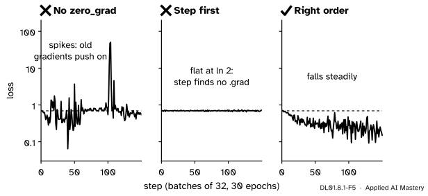
Wrong beside right on the make_moons network. Without zero_grad the old gradients keep pushing and the loss spikes. With the step before backward nothing moves. Only the right order learns.
“zero_grad is housekeeping; leaving it out only wastes a little memory.”
It changes the algorithm. The buffer then holds the sum of every gradient so far, and the step uses that sum. On a quadratic loss the parameters oscillate for ever, and on make_moons the loss jumps about and spikes far above where it started. Put one zero_grad in every iteration, anywhere between the last step and this backward.
“As long as all five lines run, their order does not matter.”
step uses whatever is in .grad at that moment. Called before backward (or after a zero_grad that follows backward), it finds the buffers set to None and skips every parameter, so the network never changes and the loss stays at its starting value, here about ln 2. With zero_grad(set_to_none=False) it would instead step with zeros, to the same effect.
“If one backward is good, calling it again is harmless.”
The first backward frees the graph, so a second one raises a RuntimeError. With retain_graph=True it runs, and adds the same gradient a second time: in the code above the weight’s .grad became \({2 \times (-23.5) = -47}\). Call backward once per loss.
Check yourself
Recall
1. Name the five lines of one iteration, in order.
Show answer
out = model(X), loss = loss_fn(out, y), optimizer.zero_grad(), loss.backward(), optimizer.step(). zero_grad may also come first; it must sit between the previous step and this backward.
2. What does loss.backward() do to a parameter’s .grad?
Show answer
It adds the partial derivative of the loss with respect to that parameter into .grad. It does not overwrite it. Afterwards it frees the graph.
3. What does optimizer.zero_grad() set the buffers to by default in PyTorch 2, and what does step do with such a parameter?
Show answer
To None. step skips a parameter whose .grad is None, so it is not moved.
4. In the worked example, what did .grad hold at step 2 when zero_grad was forgotten?
Show answer
\({(-23.5, -8)}\) plus \({(-3.875, -1.325)}\), which is \({(-27.375, -9.325)}\); the loss rose from 0.552 to about 12.09.
5. On a quadratic loss with curvature \(h\), for which learning rates does gradient descent without zero_grad settle?
Show answer
For none. The error obeys \({e_{t+1} = (2 - \eta h)e_t - e_{t-1}}\), whose roots have product 1, so it oscillates with constant size when \({0 < \eta h < 4}\) and grows when \({\eta h \ge 4}\).
Exercises
1.★ Carry the worked example (with zero_grad) one step further: from \({(w, b) = (1.36875, 0.46625)}\), find the gradient and the new parameters.
Show solution
The predictions are 1.835, 3.20375, 4.5725 and 5.94125, so the residuals are \(-0.165\), \(0.20375\), \(-0.4275\) and \(-0.05875\). Their sum is \(-0.4475\), and the residuals times \(x\) are \(-0.165\), \(0.4075\), \(-1.2825\) and \(-0.235\), with sum \(-1.275\). So
2.★★ Fix \({b = 0}\), so the loss of the four points is \({L(w) = 7.5w^2 - 23.5w + 18.5}\) with curvature \({h = 15}\) (ML01.5.1). With \({\eta = 0.05}\), by what factor does the error shrink per step in the correct loop? Without zero_grad, what is the period of the oscillation?
Show solution
Correct loop: \({e_{t+1} = (1 - \eta h)e_t = (1 - 0.75)e_t}\), so the error shrinks by a factor of 4 every step. Without zero_grad: \({\eta h = 0.75}\) lies between 0 and 4, so \({e_t = A\cos(\omega t + \varphi)}\) with \({\cos\omega = 1 - 0.75/2 = 0.625}\). Then \({\omega = \arccos 0.625 \approx 0.8957}\) radians, and the period is \({2\pi/\omega \approx 7.0}\) steps. The swings never shrink.
3.★★★ A batch of four examples is split into two halves of two. You call (loss_half / 2).backward() on each half, then step once. Show that .grad equals the gradient of the mean loss on all four, and check it on the worked example at \({(w, b) = (0, 0)}\).
Show solution
Let \(\ell_i\) be the loss of example \(i\). Each half’s mean loss is \({L_A = \tfrac12(\ell_1 + \ell_2)}\) and \({L_B = \tfrac12(\ell_3 + \ell_4)}\). Backward adds, so after both calls the buffer holds
the gradient of the mean over all four. At \((0, 0)\) the per-example gradients with respect to \(w\) are \({-2y_ix_i = -4, -12, -30, -48}\). The halves give \({\tfrac12 \cdot \tfrac12(-4 - 12) = -4}\) and \({\tfrac12 \cdot \tfrac12(-30 - 48) = -19.5}\), which add to \(-23.5\), the full-batch value. If the halves had different sizes, each would need weight \({\abs{B_j}/n}\) instead of \(\tfrac12\).
Summary card
Forward, loss, zero_grad, backward, step: and backward adds.
DL01.8.1-F1
Five lines, four stores, one update.
One iteration: \({\theta_{t+1} = \theta_t - \eta\,\vect{g}_t}\), with \({\vect{g}_t = \nabla L_t(\theta_t)}\).
backward: \({\text{grad} \leftarrow \text{grad} + \vect{g}_t}\). zero_grad: buffers to None.
No zero_grad: \({e_{t+1} = (2 - \eta h)e_t - e_{t-1}}\), which never settles.
step before backward moves nothing; backward twice raises an error.
Sources and next steps
Sources. Each was opened and checked against this lesson on 15 November 2026.
PyTorch 2.15 documentation, torch.optim.Optimizer.zero_grad: the default set_to_none=True, and that optimizers skip the step for a parameter whose gradient is None but take it when the gradient is zero.
PyTorch 2.15 documentation, Autograd mechanics: gradients are accumulated into the .grad of leaf tensors during backward(); running backward with retain_graph=False releases the saved tensors, and a second backward through the same graph raises an error unless retain_graph=True.
PyTorch 2.15 documentation, torch.optim.SGD: the update \({\theta \leftarrow \theta - \text{lr}\cdot g}\) when momentum and weight decay are zero.
Simon J. D. Prince, Understanding Deep Learning (MIT Press, 2023). Section 6.2.1 defines batches, epochs and the mini-batch update (equation 6.10); section 7.6 and figure 7.8 give a PyTorch training loop with the same five lines, zero_grad first.