\( \newcommand{\vect}[1]{\boldsymbol{\mathbf{#1}}} \newcommand{\mat}[1]{\boldsymbol{\mathbf{#1}}} \newcommand{\R}{\mathbb{R}} \newcommand{\E}{\mathbb{E}} \newcommand{\Prob}{\mathbb{P}} \newcommand{\T}{^{\top}} \newcommand{\norm}[1]{\lVert #1 \rVert} \newcommand{\abs}[1]{\lvert #1 \rvert} \newcommand{\ihat}{\mkern1mu\hat{\boldsymbol{\imath}}\mkern2mu} \newcommand{\jhat}{\mkern1mu\hat{\boldsymbol{\jmath}}\mkern2mu} \newcommand{\pd}[2]{\frac{\partial #1}{\partial #2}} \newcommand{\argmax}{\operatorname*{arg\,max}} \newcommand{\argmin}{\operatorname*{arg\,min}} \newcommand{\cdata}[1]{\class{c-data}{#1}} \newcommand{\cmodel}[1]{\class{c-model}{#1}} \newcommand{\ctruth}[1]{\class{c-truth}{#1}} \newcommand{\cgrad}[1]{\class{c-grad}{#1}} \newcommand{\closs}[1]{\class{c-loss}{#1}} \newcommand{\cparam}[1]{\class{c-param}{#1}} \newcommand{\csecond}[1]{\class{c-second}{#1}} \renewcommand{\,}{\mkern3mu} \)

Binary cross-entropy from the Bernoulli

A sigmoid output is the bias of a coin. Its negative log-likelihood is the log loss, which in terms of the logit is softplus(-z) or softplus(z): the form libraries compute, because it never takes the log of zero. Its gradient is p - y, and it does not vanish when the model is confidently wrong.

DL01.4.2L2 Intermediate25 min

In review (what this means)

The maths and code on this page are checked by automated tests on every change, but an independent reader has not signed it off yet. Spot a mistake or a confusing step? Tell us.

Before this lesson: DL01.4.1 Regression losses as noise models ML01.6 Logistic regression and classification

What you will be able to do

• Derive binary cross-entropy as the negative log-likelihood of a Bernoulli label whose parameter is a sigmoid output.
• Rewrite the loss in terms of the logit as softplus(-z) for y = 1 and softplus(z) for y = 0, and compute it without overflow.
• Derive the gradient p - y with respect to the logit, and compare it with the gradient 2 (p - y) p (1 - p) of squared error after a sigmoid.
• Show with numbers why the naive formula fails at z = 40 and why clipping probabilities hides the true loss.

The question

The last neuron of a classifier outputs a number \(z\), the logit, and the sigmoid turns it into a probability. For one example labelled 0 the network says \({z = 40}\): it is almost certain of the wrong answer. Compute the log loss of ML01.6.2 in the obvious way, \({-\ln(1 - \sigma(z))}\), in 64-bit floating point, and you get infinity; one such example turns a whole training run into nan. The true loss is 40. Where does this loss come from, and how should it be computed?

From the last lesson

1. In the maximum-likelihood recipe, what does the network output, and what is the loss?

Show answer

The parameters of a distribution over the target; the loss is the mean of minus the log probability (or density) that distribution gives to each observed target.

2. Which noise distribution gives the mean squared error, and which gives the mean absolute error?

Show answer

A Gaussian of fixed variance gives the mean squared error; a Laplace distribution gives the mean absolute error.

Intuition

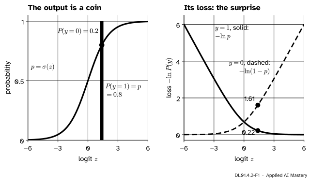
For a yes-or-no target the “bell” of lesson 1 becomes a coin. The network’s output, after the sigmoid, is the coin’s bias: the probability \(p\) that the label is 1. The probability of a 0 is whatever is left, \({1 - p}\). The recipe has not changed: the loss is the surprise, minus the log of the probability the coin gave to the label that was actually seen.

DL01.4.2-F1

Left: the logit \({z = \ln 4}\) gives the coin bias \({p = 0.8}\). Right: the loss if the label turns out to be 1 (solid) or 0 (dashed). Seeing a 1 costs \({-\ln 0.8 = 0.22}\); seeing a 0 costs \({-\ln 0.2 = 1.61}\).

Both curves have the same shape, mirrored. Far on the side where the model is right, the loss is nearly 0. Far on the side where it is wrong, the loss grows like a straight line: twice as wrong a logit costs about twice as much. That straight-line growth is what keeps learning alive.

Build it up

Step 1. The coin as a formula. A Bernoulli distribution with parameter \(p\) gives a label \({y \in \{0, 1\}}\) the probability

\[ P(y \mid p) = p^{\,y}\,(1 - p)^{1 - y}. \]

Check both cases: \({y = 1}\) gives \({p^1 (1-p)^0 = p}\), and \({y = 0}\) gives \({p^0 (1-p)^1 = 1 - p}\). The exponents simply switch the right factor on.

Step 2. Minus its log. The log turns the product into a sum and brings the exponents down:

\[ \begin{aligned} \ell &= -\ln P(y \mid p) \\ &= -\big[\,y \ln p + (1 - y)\ln(1 - p)\,\big]. \end{aligned} \]

This is the binary cross-entropy, the same log loss as ML01.6.2. The recipe of lesson 1 has rebuilt it without any new idea.

Step 3. Write it with the logit. The network computes \(z\), and \({p = \sigma(z) = 1/(1 + e^{-z})}\). For a label 1,

\[ \begin{aligned} -\ln \sigma(z) &= -\ln \frac{1}{1 + e^{-z}} \\ &= \ln(1 + e^{-z}). \end{aligned} \]

For a label 0 we need \({1 - \sigma(z)}\). Multiply the top and bottom of \({e^{-z}/(1 + e^{-z})}\) by \(e^{z}\):

\[ \begin{aligned} 1 - \sigma(z) &= \frac{e^{-z}}{1 + e^{-z}} \\ &= \frac{1}{e^{z} + 1} = \sigma(-z), \end{aligned} \]

so \({-\ln(1 - \sigma(z)) = \ln(1 + e^{z})}\). The function \({\ln(1 + e^{z})}\) is the softplus, met in DL01.3.3. The two cases are

\[ \ell(z, y) = \begin{cases} \mathrm{softplus}(-z) & y = 1, \\ \mathrm{softplus}(z) & y = 0. \end{cases} \]

Step 4. One formula for both. Subtracting \(z\), which is \({\ln e^{z}}\), from the softplus gives the softplus of \({-z}\):

\[ \begin{aligned} &\mathrm{softplus}(z) - z \\ &\quad= \ln(1 + e^{z}) - \ln e^{z} \\ &\quad= \ln(e^{-z} + 1) = \mathrm{softplus}(-z). \end{aligned} \]

So both cases are

\[ \ell(z, y) = \mathrm{softplus}(z) - y\,z . \]

DL01.4.2-F2

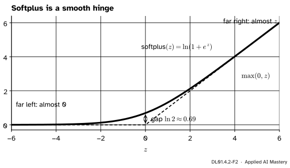
Softplus is a smooth hinge: never more than \({\ln 2}\) above \({\max(0, z)}\), and almost on it a few units away. So a confidently wrong logit costs about \({|z|}\).

Step 5. Compute it safely. For \({z \ge 0}\), factor \(e^{z}\) out of the bracket:

\[ \begin{aligned} \ln(1 + e^{z}) &= \ln\big(e^{z}(e^{-z} + 1)\big) \\ &= z + \ln(1 + e^{-z}). \end{aligned} \]

For \({z < 0}\) the original form is already safe. Together,

\[ \begin{aligned} &\mathrm{softplus}(z) \\ &\quad= \max(z, 0) + \ln\big(1 + e^{-|z|}\big). \end{aligned} \]

The exponential now only ever sees \({-|z| \le 0}\), so it can never overflow, and nothing is ever the log of 0.

The formal statement

NoteBinary cross-entropy and its gradient

For a label \({\ctruth{y} \in \{0, 1\}}\) and a logit \(\cmodel{z}\) with \({\cmodel{p} = \sigma(\cmodel{z})}\),

\[ \begin{aligned} \closs{\ell} &= \mathrm{softplus}(\cmodel{z}) - \ctruth{y}\,\cmodel{z}, \\ \cgrad{\pd{\ell}{z}} &= \cmodel{p} - \ctruth{y}. \end{aligned} \]

The gradient. The derivative of the softplus is the sigmoid:

\[ \begin{aligned} \frac{d}{dz}\ln(1 + e^{z}) &= \frac{e^{z}}{1 + e^{z}} \\ &= \frac{1}{e^{-z} + 1} = \sigma(z), \end{aligned} \]

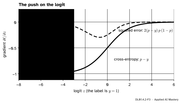
where the middle step divides top and bottom by \(e^{z}\). The derivative of \({-yz}\) is \({-y}\). So \({\partial \ell / \partial z = \sigma(z) - y = p - y}\): prediction minus label. Its size is the size of the mistake. A model that gives \({p = 0.007}\) to a true 1 gets a push of \({-0.993}\), almost the largest possible.

Squared error after a sigmoid. Suppose instead the loss were \({(p - y)^2}\), as if the probability were a regression target. By the chain rule, with \({\sigma' = \sigma(1 - \sigma)}\) from DL01.3.1,

\[ \begin{aligned} \pd{}{z}(p - y)^2 &= 2(p - y)\,\frac{dp}{dz} \\ &= 2(p - y)\,p\,(1 - p). \end{aligned} \]

The extra factor \({p(1 - p)}\) is near 0 whenever \(p\) is near 0 or 1, whether the model is right or badly wrong. When it is confidently wrong, the gradient vanishes just when it is needed most.

DL01.4.2-F3

The push on the logit for an example with label 1. Cross-entropy pushes with nearly full strength when the model is confidently wrong; squared error has almost stopped pushing.

Worked example

A confident mistake. The label is \({y = 1}\) and the logit is \({z = -5}\). Then \({e^{5} = 148.41}\), so \({p = 1/149.41 = 0.00669}\).

• Cross-entropy: \(\mathrm{softplus}(5) = 5 + {\ln(1 + e^{-5})} = 5 + 0.00672 = 5.007\). Its gradient is \({p - y = -0.993}\).
• Squared error: \({(p - y)^2 = 0.993^2 = 0.987}\). Its gradient is \({2(-0.993)(0.00669)(0.993)} = -0.0132\).

With the same learning rate, cross-entropy moves the logit about 75 times as far.

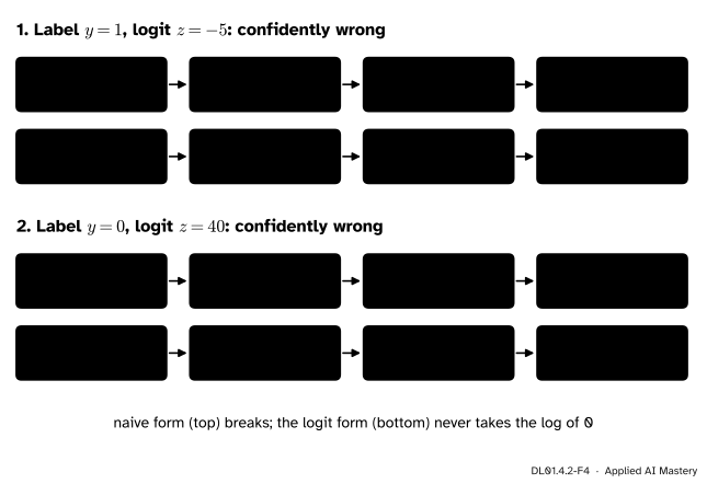
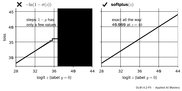
A confident wrong answer, computed two ways. The label is \({y = 0}\) and \({z = 40}\). In exact arithmetic \(1 - {\sigma(40)} = {\sigma(-40)} \approx {4.2 \times 10^{-18}}\). In 64-bit floating point, \({1 + e^{-40}}\) rounds to exactly 1, because the gap between 1 and the next number is about \({2.2 \times 10^{-16}}\). So \(\sigma(40)\) comes out as exactly \({1.0}\), \({1 - p = 0}\) and \({-\ln 0 = \infty}\). The logit form never forms \({1 - p}\): \(\mathrm{softplus}(40) = 40 + {\ln(1 + e^{-40})} = 40.000\).

DL01.4.2-F4

Both computations of the worked example, box by box.

Code

From scratch: the naive formula, the logit form, and both gradients, checked by central differences.

import numpy as np

def sigmoid(z):
    return 1 / (1 + np.exp(-z))

def bce_naive(z, y):
    p = sigmoid(z)
    return -(y * np.log(p) + (1 - y) * np.log(1 - p))

def softplus(z):
    return np.maximum(z, 0) + np.log1p(np.exp(-np.abs(z)))

def bce_logits(z, y):
    return softplus(z) - y * z

z, y = -5.0, 1.0
p = sigmoid(z)
g_ce, g_se = p - y, 2 * (p - y) * p * (1 - p)
h = 1e-6
numeric_ce = (bce_logits(z + h, y) - bce_logits(z - h, y)) / (2 * h)
numeric_se = ((sigmoid(z + h) - y) ** 2 - (sigmoid(z - h) - y) ** 2) / (2 * h)
print(f"p = {p:.5f}  cross-entropy {bce_logits(z, y):.3f}, gradient {g_ce:.4f} (numeric {numeric_ce:.4f})")
print(f"squared error {(p - y) ** 2:.3f}, gradient {g_se:.4f} (numeric {numeric_se:.4f})")
print(f"ratio of the two pushes: {g_ce / g_se:.0f}")

with np.errstate(divide="ignore"):
    naive = bce_naive(40.0, 0.0)
print("z = 40, y = 0:  naive", naive, "  logit form", bce_logits(40.0, 0.0))

p = 0.00669  cross-entropy 5.007, gradient -0.9933 (numeric -0.9933)
squared error 0.987, gradient -0.0132 (numeric -0.0132)
ratio of the two pushes: 75
z = 40, y = 0:  naive inf   logit form 40.0

scikit-learn’s log_loss takes probabilities, not logits. On ordinary values it agrees with our mean:

from sklearn.metrics import log_loss

zs = np.array([-5.0, 0.5, 2.0, -1.0])
ys = np.array([1.0, 0.0, 1.0, 0.0])
print("ours:", round(float(np.mean(bce_logits(zs, ys))), 6), " scikit-learn:", round(log_loss(ys, sigmoid(zs)), 6))
print("z = 40, y = 0 through probabilities:", round(log_loss([0], [sigmoid(40.0)], labels=[0, 1]), 2))

ours: 1.605246  scikit-learn: 1.605246
z = 40, y = 0 through probabilities: 36.04

Handed \({p = 1.0}\), scikit-learn clips it to \({1 - \epsilon}\), with \(\epsilon\) the machine epsilon \({2.2 \times 10^{-16}}\), and reports \({-\ln \epsilon = 36.04}\) instead of the true 40. That is the best a function can do once the logit has been thrown away. Deep-learning libraries therefore offer a loss that takes the logit itself; DL01.7.4 meets PyTorch’s.

Explore

DL01.4-X1

One-example loss explorer

It opens on the worked example, \({y = 1}\) and \({z = -5}\). Press each Step button and compare how far one step moves the logit. Then slide \(z\) to the right, set the label to 0, and switch to three classes for the softmax of the next lesson.

Pitfalls

DL01.4.2-F5

Wrong beside right. Computed through the probability, the loss turns into a staircase and then infinity once \({\sigma(z)}\) rounds to 1, near \({z = 36.7}\). Computed from the logit, it is exact.

“Apply the sigmoid, then take the log loss: it is the same thing.”

It is the same in exact arithmetic, not in floating point. Once \({\sigma(z)}\) is rounded, the information that separates \({z = 37}\) from \({z = 40}\) is gone, and the log of a rounded \({1 - p}\) is either coarse or infinite. Keep the logit and compute \({\mathrm{softplus}(z) - yz}\).

“Squared error on the probability is fine: it is still smallest at the right answer.”

Its minimum is in the right place, but the road there is flat exactly where the model is most wrong: a push of \({-0.013}\) instead of \({-0.993}\) at \({z = -5}\). A network that starts out confidently wrong on some examples can sit there for a long time.

“Clipping the probabilities to \({[\epsilon, 1 - \epsilon]}\) solves the problem.”

It stops the infinity but caps the loss at \({-\ln \epsilon}\), 36.04 in 64-bit floats, and the loss is flat beyond the clip, so its gradient there is 0. A confidently wrong example then teaches nothing.

Check yourself

Recall

1. Write the Bernoulli probability of a label \(y\) with parameter \(p\), and check both values of \(y\).

Show answer

\({P(y \mid p) = p^{y}(1 - p)^{1 - y}}\). For \({y = 1}\) it is \(p\); for \({y = 0}\) it is \({1 - p}\).

2. Write binary cross-entropy in terms of the logit for \({y = 1}\), for \({y = 0}\), and as one formula.

Show answer

\({\mathrm{softplus}(-z)}\), \({\mathrm{softplus}(z)}\), and \({\mathrm{softplus}(z) - yz}\), where \({\mathrm{softplus}(z) = \ln(1 + e^{z})}\).

3. What is the gradient of binary cross-entropy with respect to the logit?

Show answer

\({p - y}\), the predicted probability minus the label.

4. What is the gradient of \({(p - y)^2}\) with respect to the logit, and why does it vanish when the model is confidently wrong?

Show answer

\({2(p - y)p(1 - p)}\). When the model is confident, \(p\) is near 0 or 1, so \({p(1 - p)}\) is near 0, whichever label is true.

5. Why does \({-\ln(1 - \sigma(40))}\) come out as infinity in 64-bit floating point?

Show answer

\({1 + e^{-40}}\) rounds to exactly 1, so \({\sigma(40)}\) is exactly 1.0, \({1 - p}\) is 0, and \({-\ln 0}\) is infinite. The true value is about 40.

Exercises

1. ★ A model gives \({z = 2}\) to an example. Find \(p\), the loss and the gradient with respect to \(z\) if the label is 1, and again if it is 0.

Show solution

\(p = {\sigma(2)} = 0.881\). Label 1: loss \(\mathrm{softplus}(-2) = {\ln(1 + e^{-2})} = 0.127\), gradient \({0.881 - 1 = -0.119}\). Label 0: loss \(\mathrm{softplus}(2) = 2 + 0.127 = 2.127\), gradient \({0.881}\).

2. ★★ Show that \({\mathrm{softplus}(z) - \mathrm{softplus}(-z) = z}\) for every \(z\), and use it to check that \({\mathrm{softplus}(z) - yz}\) gives the right loss for \({y = 1}\).

Show solution

The difference of two logs is the log of a quotient:

\[ \begin{aligned} &\mathrm{softplus}(z) - \mathrm{softplus}(-z) \\ &\quad= \ln\frac{1 + e^{z}}{1 + e^{-z}}. \end{aligned} \]

The top is \(1 + e^{z} = {e^{z}(e^{-z} + 1)}\), so the quotient is \(e^{z}\) and its log is \(z\). Then for \({y = 1}\), \({\mathrm{softplus}(z) - z} = {\mathrm{softplus}(-z)} = {-\ln\sigma(z)}\), as it should be.

3. ★★★ For a label 1, find the logit at which the squared-error gradient \({2(p - 1)p(1 - p)}\) is largest in size, and the size there. (Hint: write it as a function of \(p\).)

Show solution

In size the gradient is \({g(p) = 2p(1 - p)^2}\) for \({0 < p < 1}\). Its derivative is \({2(1 - p)^2} - {4p(1 - p)} = {2(1 - p)(1 - 3p)}\), zero at \({p = \tfrac13}\). There \(g = {2 \cdot \tfrac13 \cdot \tfrac49} = \tfrac{8}{27} \approx 0.296\), at the logit \(z = {\ln\frac{p}{1-p}} = {\ln\tfrac12} \approx -0.693\). So squared error never pushes the logit harder than 0.296, while cross-entropy pushes with up to 1.

Summary card

The sigmoid output is a coin; the loss is the surprise of the label seen.

DL01.4.2-F1

A coin, and the cost of its surprise.

• Bernoulli: \({P(y \mid p) = p^{y}(1 - p)^{1 - y}}\), with \({p = \sigma(z)}\).
• Loss: \({\ell = \mathrm{softplus}(z) - yz}\), never taking the log of 0.
• Safe softplus: \({\max(z, 0) + \ln(1 + e^{-|z|})}\).
• Gradient: \({\partial\ell/\partial z = p - y}\); squared error gives \({2(p - y)p(1 - p)}\), which vanishes when confidently wrong.

Sources and next steps

Sources. Each was opened and checked against this lesson on 15 November 2026.

• Simon J. D. Prince, Understanding Deep Learning, MIT Press, 2023 (free PDF). Section 5.4 chooses the Bernoulli distribution (equations 5.16 and 5.17), passes the network output through the logistic sigmoid (5.18) and obtains the binary cross-entropy loss (5.20).
• Ian Goodfellow, Yoshua Bengio and Aaron Courville, Deep Learning, MIT Press, 2016. Section 6.2.2.2 rewrites the loss of a sigmoid output with the softplus function (equations 6.24 to 6.26), notes that it saturates only when the answer is already right, and that its gradient does not shrink for an extremely wrong \(z\).
• scikit-learn 1.9 documentation, sklearn.metrics.log_loss. The formula with the natural log, and the clipping of the probabilities to \({[\epsilon, 1 - \epsilon]}\) with \(\epsilon\) the machine precision of their dtype.

Next. DL01.4.3 Softmax and categorical cross-entropy replaces the coin with a die of \(K\) faces.

This lesson unlocks

DL01.4.3 Softmax and categorical cross-entropy

Your progress is saved in this browser only. No account, no tracking.