When a value feeds two places, the gradients coming back add. Work it on a network with two output heads, a skip connection and a weight used twice, then see concatenation split a gradient and a sum broadcast it back, and catch the overwrite bug.
DL01.5.3L2 Intermediate25 minIn review (what this means)
The maths and code on this page are checked by automated tests on every change, but an independent reader has not signed it off yet. Spot a mistake or a confusing step? Tell us.
State the fork rule, that the gradient of a value used in several places is the sum of the gradients from each use, and derive it from the multivariable chain rule.
Backpropagate by hand through a network with two output heads and a summed loss, and through a skip connection.
Compute the gradient of a weight that is used twice as the sum over its uses.
Explain why concatenation splits a gradient and a sum broadcasts it, and spot the bug of overwriting a gradient instead of adding to it.
The question
Real networks are not chains. A multi-task model reads its input with one shared trunk and feeds the result to several heads, each with its own loss. Residual networks add a layer’s input to its output. Some language models use the same matrix to read words in and to write them out. In each, one value is used in two places. Which gradient does it get back, and what happens if the code keeps only one of them?
From the last lesson
1. What does a Linear module return from backward, and what does it store?
Show answer
It returns \({\mat{G}\mat{W}}\), the gradient of its input, and stores \({\mat{G}\T\mat{A}}\) and the column sums of \(\mat{G}\), the gradients of its weights and bias.
2. Where does the factor \(1/n\) in the backward pass of a mean loss enter?
Show answer
Once, at the top: the loss module returns \({(\mat{P} - \mat{Y})/n}\), and every gradient below inherits it.
Intuition
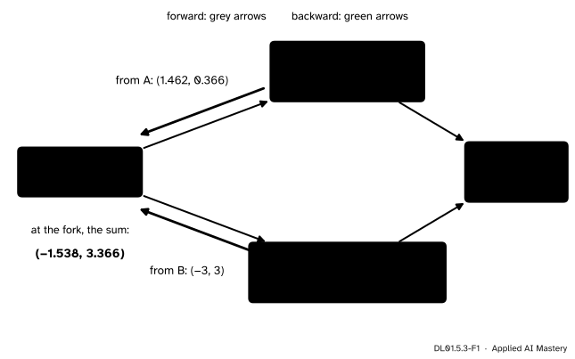
Give the running network of DL01.5.1 a second head. Its hidden activations \(\vect{a}^{(1)}\) now feed head A, the classifier, and head B, which predicts a number from the same features. The total loss is the sum of the two heads’ losses.
DL01.5.3-F1
One value, two uses. Each head sends back its own gradient, and the gradient of \(\vect{a}^{(1)}\) is their sum. Nudge \(\vect{a}^{(1)}\) and both losses move; the total change is the change through A plus the change through B.
That is the whole lesson: at a fork, gradients add. Whenever a value has several children in the graph, its gradient is the sum of what each child sends back. The rule is not new. Every dense layer already used it: each \(a_j\) feeds every output unit, and \({\mat{W}\T\vect{\delta}}\) sums those contributions (DL01.5.1). Branches, skips and shared weights are the same rule in plain sight.
Build it up
Step 1. Head B. It is a single linear unit, \({\hat{y}_B} = {\vect{v}\T\vect{a}^{(1)} + b_B}\) with \({\vect{v}} = {(1, -1)}\) and \({b_B} = {0}\), trained on the target \({y_B} = {1}\) with the squared error \({L_B} = {(\hat{y}_B - y_B)^2}\). Here \({\hat{y}_B} = {0.5 - 1} = {-0.5}\) and \({L_B} = {2.25}\).
Step 2. Each head’s gradient at the fork. Head A sends back what it sent in DL01.5.1, \({\mat{W}^{(2)\top}\vect{\delta}^{(2)}} = {(1.462, 0.366)}\). Head B has \({\partial L_B/\partial\hat{y}_B} = {2(\hat{y}_B - y_B)} = {-3}\), and its multiply node sends \({\vect{v} \times (-3)} = {(-3, 3)}\).
Step 3. Add.\({\partial L/\partial\vect{a}^{(1)}} = {(1.462 - 3,\; 0.366 + 3)} = {(-1.538, 3.366)}\). From here the trunk is the old chain: the mask, then the first layer.
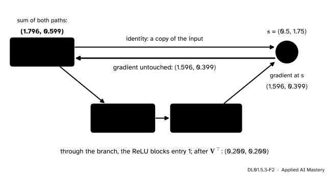
Step 4. A skip. A residual block adds its input to the output of a small branch, \({\vect{s}} = {\vect{a}^{(1)} + \operatorname{relu}(\mat{V}\vect{a}^{(1)})}\). The value \(\vect{a}^{(1)}\) feeds two children: the add node directly, and the branch.
DL01.5.3-F2
A skip is a fork followed by an add. The add node copies the gradient into both paths, so the identity path hands it back untouched, and the branch adds whatever gets through it.
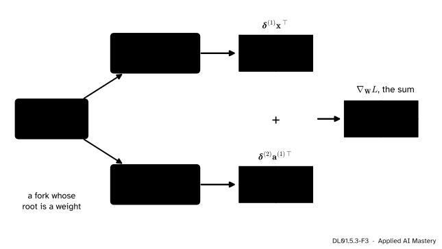
Step 5. A weight used twice. Tie the two layers of the running network together, so that the same matrix \(\mat{W}\) plays \(\mat{W}^{(1)}\) and \(\mat{W}^{(2)}\). Imagine two copies, \({\mat{W}_1} = {\mat{W}}\) and \({\mat{W}_2} = {\mat{W}}\), made by a fork. Each copy gets the gradient of its own layer, and the fork adds them.
DL01.5.3-F3
A shared weight is a fork in the graph whose root is the parameter. Its gradient is the sum of the gradients it would get if each use had its own copy.
The formal statement
NoteThe fork rule
If a value \(v\) is used by children \({u_1, \dots, u_m}\) of the graph, then
In code: every child adds its contribution into the gradient of \(v\), starting from zero.
Why.\(L\) depends on \(v\) only through its children. Write \({L} = {f(u_1(v), \dots, u_m(v))}\) and apply the multivariable chain rule (M05.4.2): the rate of change is one product per path, summed over the paths. Goodfellow and colleagues write the same rule as \({\partial z/\partial x_i} = {\sum_j (\partial z/\partial y_j)(\partial y_j/\partial x_i)}\), their equation 6.45.
Four special cases cover every graph in this course.
A sum of losses.\({L} = {L_A + L_B}\) is an add node, so each head receives the gradient 1 at its loss, as if it were alone. The heads then meet again at the fork.
A skip.\({\vect{s}} = {\vect{a} + g(\vect{a})}\) gives \({\partial L/\partial\vect{a}} = {\vect{g}_s + \mat{J}_g\T\vect{g}_s}\), where \(\vect{g}_s\) is the gradient at \(\vect{s}\) and \(\mat{J}_g\) the Jacobian of the branch. The first term never vanishes, whatever the branch does; why that matters in deep networks is DL02.7.
A shared weight. With uses \({\mat{W}_1} = {\mat{W}_2} = {\mat{W}}\), \({\nabla_{\mat{W}}L} = {\nabla_{\mat{W}_1}L + \nabla_{\mat{W}_2}L}\).
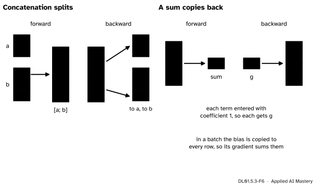
Concatenation and sum. They are each other’s backward, and so are copying and summing.
DL01.5.3-F6
Concatenation splits the gradient back into the pieces it came from. A sum sends the same gradient to every term, because each term enters with coefficient 1. In a batch, the bias is copied into every row on the way forward, so its gradient sums the rows on the way back.
Concatenation.\({\vect{c}} = {[\vect{a};\, \vect{b}]}\) copies each entry of \(\vect{a}\) and \(\vect{b}\) to one place in \(\vect{c}\), so \({\partial L/\partial a_i} = {\partial L/\partial c_i}\) for the first block and likewise for \(\vect{b}\) with the rest. Sum.\({s} = {\sum_i v_i}\) has \({\partial s/\partial v_i} = {1}\), so every \(v_i\) gets \({\partial L/\partial s}\).
Worked example
The two-head network, every number. The forward pass of the trunk is that of DL01.5.1: \({\vect{z}^{(1)}} = {\vect{a}^{(1)}} = {(0.5, 1)}\).
DL01.5.3-F4
The two heads work independently until the fork, where their gradients add; below the fork there is one trunk and one backward pass.
Head A. Unchanged from DL01.5.1: loss 1.313, gradients of \(\mat{W}^{(2)}\) and \(\vect{b}^{(2)}\) as before, and \({(1.462, 0.366)}\) sent to the fork.
Head B.\({\partial L_B/\partial\hat{y}_B} = {-3}\). The multiply node swaps: the weights get \({-3 \times \vect{a}^{(1)}} = {(-1.5, -3)}\), the bias gets \(-3\), and the fork gets \({-3 \times \vect{v}} = {(-3, 3)}\).
The trunk. At the fork, \({(-1.538, 3.366)}\). Both units are on, so \({\vect{\delta}^{(1)}} = {(-1.538, 3.366)}\), and \({\nabla_{\mat{W}^{(1)}}L} = {\vect{\delta}^{(1)}\vect{x}\T}\) has rows \({(-1.538, -3.076)}\) and \({(3.366, 6.731)}\). The total loss is \({1.313 + 2.25} = {3.563}\).
Compare with DL01.5.1, where \({\nabla_{\mat{W}^{(1)}}L}\) had rows \({(1.462, 2.924)}\) and \({(0.366, 0.731)}\). Head B pulls the first hidden unit the other way: it wants \({a^{(1)}_1}\) larger (its weight in \(\vect{v}\) is \(+1\) and its prediction is too low), while head A wants it smaller. The trunk serves both, and the sum decides.
Code
The modules of DL01.5.2, unchanged, are in the folded cell. New code only wires them together.
loss 3.563  from A [[1.462 0.366]]  from B [[-3.  3.]]
grad W1 = [[-1.538, -3.076], [3.366, 6.731]]
A skip, and a weight used twice. For the skip, a small Residual module adds the two paths in its backward. For the tied network, two Linear modules share one array, and the gradient of that array is the sum of the two stored gradients.
class Residual:"""s = a + branch(a); the backward adds the identity path and the branch path."""def__init__(self, *branch):self.branch = branchdef forward(self, A): out = Afor m inself.branch: out = m.forward(out)return A + outdef backward(self, G): g = Gfor m inreversed(self.branch): g = m.backward(g)return G + glin1, relu = Linear(W1, b1), ReLU()skip, head = Residual(Linear([[1, -1], [0.5, 0.5]], [0, 0]), ReLU()), Linear(W2, b2)ce = SoftmaxCrossEntropy()ce.forward(head.forward(skip.forward(relu.forward(lin1.forward(X)))), label)g_s = head.backward(ce.backward())g_a1 = skip.backward(g_s)print("gradient at s", g_s.round(3), " at a1", g_a1.round(3))W = np.array(W1, float) # one array, used by both layersfirst, second = Linear(W, b1), Linear(W, b2)first.W = second.W = Wce, r = SoftmaxCrossEntropy(), ReLU()loss_tied = ce.forward(second.forward(r.forward(first.forward(X))), label)first.backward(r.backward(second.backward(ce.backward())))grad_W = first.dW + second.dW # sum over the two usesprint("use in layer 1", first.dW.round(3).tolist(), " use in layer 2", second.dW.round(3).tolist())
gradient at s [[1.596 0.399]]   at a1 [[1.796 0.599]]
use in layer 1 [[0.334, 0.668], [-0.334, -0.668]]   use in layer 2 [[0.111, 0.223], [-0.111, -0.223]]
Central differences settle all three cases, and show the overwrite bug for what it is.
def softmax_ce(z, k): z = z - z.max()return-(z[k] - np.log(np.exp(z).sum()))def loss_heads(w): a = np.maximum(w @ X[0] + b1, 0)return softmax_ce(np.array(W2) @ a + b2, 1) + (a[0] - a[1] -1.0) **2def loss_tied_of(w): a = np.maximum(w @ X[0] + b1, 0)return softmax_ce(w @ a + b2, 1)def numeric(f, w, h=1e-5): out = np.zeros_like(w)for idx in np.ndindex(w.shape): e = np.zeros_like(w); e[idx] = h out[idx] = (f(w + e) - f(w - e)) / (2* h)return outw0 = np.array(W1, float)print("two heads, add: ", f"{np.abs(numeric(loss_heads, w0) - two_heads()[3]).max():.1e}")print("two heads, overwrite:", f"{np.abs(numeric(loss_heads, w0) - two_heads(overwrite=True)[3]).max():.1e}")print("tied weights, sum: ", f"{np.abs(numeric(loss_tied_of, w0) - grad_W).max():.1e}")
two heads, add:       8.7e-11
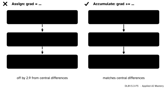
two heads, overwrite: 2.9e+00
tied weights, sum:    9.6e-11
The overwrite version is off by more than 1 on a gradient whose entries are at most about 7: not a rounding error, a lost head.
Explore
The Backprop stepper in DL01.5.1 shows the fork rule inside an ordinary dense layer. Step to backward step 3, where each hidden activation receives the gradient from both logits. Set \({w^{(2)}_{11}}\) to 0 and watch the first hidden unit’s gradient come from logit 2 alone.
Pitfalls
DL01.5.3-F5
Wrong beside right. With an assignment, whichever branch runs last wins and the other head is forgotten. Only adding gives the gradient of the total loss.
“Each branch sets the gradient of the value it reads.”
If the code writes grad = from_b after grad = from_a, head A vanishes from the backward pass. The first layer then trains only for head B, and nothing crashes. Gradients of shared values must be accumulated: start at zero and add. This is why autodiff engines and PyTorch add into .grad (DL01.6.3, DL01.8.1).
“A tied weight needs only the gradient of one of its uses.”
For the tied network the use in layer 1 gives rows \({(0.334, 0.668)}\) and \({(-0.334, -0.668)}\); the true gradient is the sum with layer 2’s contribution, rows \({(0.445, 0.891)}\) and \({(-0.445, -0.891)}\). Keeping one use updates the shared matrix as if the other did not exist.
“A skip connection skips the backward pass too.”
It skips nothing: the skip adds a path, it does not remove one. The branch still gets its gradient and its weights still learn; the identity path simply delivers \({\vect{g}_s}\) to the input as well. In the example the branch’s first unit is off, yet \({\vect{a}^{(1)}}\) still receives \({(1.796, 0.599)}\).
Check yourself
Recall
1. State the fork rule.
Show answer
If a value feeds several children, its gradient is the sum over the children of each child’s gradient times the local derivative of that child with respect to the value.
2. What does each head receive at its own loss when the total loss is \({L_A + L_B}\)?
Show answer
A gradient of 1, because the sum is an add node, which copies the gradient to both inputs.
3. What is the gradient of a weight that is used twice?
Show answer
The sum of the gradients of its two uses, as if each use had its own copy.
4. What is the backward of concatenation, and of a sum?
Show answer
Concatenation splits the incoming gradient into the pieces that were joined. A sum copies its gradient to every term.
5. Through a skip \({\vect{s}} = {\vect{a} + g(\vect{a})}\), what reaches \(\vect{a}\) even if the branch passes nothing back?
Show answer
The gradient at \(\vect{s}\) itself, through the identity path.
Exercises
1.★ In the two-head network, change head B’s target to \({y_B} = {-0.5}\). What does head B send back, and what is the gradient at the fork?
Show solution
Now \({\hat{y}_B} = {-0.5} = {y_B}\), so \({L_B} = {0}\) and \({\partial L_B/\partial\hat{y}_B} = {2(\hat{y}_B - y_B)} = {0}\). Head B sends back \({(0, 0)}\), and the fork holds head A’s gradient alone, \({(1.462, 0.366)}\): a head that is already right has nothing to say.
2.★★ A loss is \({L} = {(w x)^2 + w}\) for one number \(w\) and input \({x} = {3}\). Draw \(w\) as a value with two children, find \({dL/dw}\) by the fork rule, and check it by differentiating directly. Evaluate it at \({w} = {0.5}\).
Show solution
The children of \(w\) are \({u_1} = {wx}\), which feeds the square, and \({u_2} = {w}\) itself, added at the end. Path 1: \({\partial L/\partial u_1} = {2u_1} = {2wx}\) and \({\partial u_1/\partial w} = {x}\), giving \({2wx^2}\). Path 2: \({\partial L/\partial u_2} = {1}\) with local derivative 1. Sum: \({2wx^2 + 1}\). Directly, \({L} = {w^2x^2 + w}\) has derivative \({2wx^2 + 1}\), the same. At \({w} = {0.5}\), \({x} = {3}\): \({2 \times 0.5 \times 9 + 1} = {10}\). This is Figure 6.8(d) of Goodfellow and colleagues in miniature: a weight used in a prediction and in a penalty.
3.★★★ A layer reads \({\vect{c}} = {[\vect{a};\, \vect{x}]}\), the hidden activations stacked on the raw input, through weights \(\mat{U}\) of shape (2, 4): \({\vect{z}} = {\mat{U}\vect{c}}\). Show that the gradient reaching \(\vect{a}\) is \({\mat{U}_a\T\vect{\delta}}\), where \(\mat{U}_a\) is the first two columns of \(\mat{U}\), and say what reaches \(\vect{x}\).
Show solution
The dense-layer rule gives \({\partial L/\partial\vect{c}} = {\mat{U}\T\vect{\delta}}\), a vector of length 4. Write \({\mat{U}} = {[\mat{U}_a \;\; \mat{U}_x]}\) in blocks of two columns. Then \({\mat{U}\vect{c}} = {\mat{U}_a\vect{a} + \mat{U}_x\vect{x}}\), and \({\mat{U}\T\vect{\delta}}\) stacks \({\mat{U}_a\T\vect{\delta}}\) on top of \({\mat{U}_x\T\vect{\delta}}\). Concatenation splits this: \(\vect{a}\) receives the first block, \({\mat{U}_a\T\vect{\delta}}\), and \(\vect{x}\) the second, \({\mat{U}_x\T\vect{\delta}}\). If \(\vect{x}\) also fed the first layer, the fork rule would add this to what comes back through that layer.
Shared weight: sum over its uses. Concatenation splits; a sum copies back.
Sources and next steps
Sources. Each was opened and checked against this lesson on 15 November 2026.
Stanford CS231n, Backpropagation, Intuitions. “Gradients add up at forks”: if a variable branches out to different parts of the circuit, the gradients that flow back to it add, following the multivariable chain rule.
I. Goodfellow, Y. Bengio and A. Courville, Deep Learning (MIT Press, 2016), section 6.5.2: the chain rule for vectors, equations 6.45 and 6.46. Figure 6.8(d) shows a graph in which the weights are used both for the prediction and for the weight-decay penalty.
S. J. D. Prince, Understanding Deep Learning (MIT Press, 2023), section 7.4.3: the ideas of backpropagation still hold for branching graphs, such as a hidden layer processed by two sub-networks and recombined, as long as the graph is acyclic.