Put the hand-built module library to work: forward, loss, backward and a gradient step for every parameter, in mini-batches over the two moons, until a 2-16-16-2 network bends its decision boundary around the data, with a validation loss beside the training loss.
DL01.5.4L2 Intermediate25 minIn review (what this means)
The maths and code on this page are checked by automated tests on every change, but an independent reader has not signed it off yet. Spot a mistake or a confusing step? Tell us.
Write a mini-batch gradient-descent loop around the module library: shuffle, forward, loss, backward, update.
Carry out one gradient step on the running network by hand and predict the fall in the loss to first order.
Train a 2-16-16-2 network on the two moons and read its training and validation curves.
Compare the hand-built loop with scikit-learn’s MLPClassifier and name what the library adds by default.
The question
Three lessons of gradients, and not one step of learning yet. The module library can now compute the gradient of any loss with respect to every weight of a stack of layers. Is that enough to train a real network? Take the two moons, which no straight line can separate, and a network with 354 parameters: can a page of hand-written NumPy bend its decision boundary around them in a few seconds?
From the last lesson
1. A value feeds two heads. What is its gradient?
Show answer
The sum of the gradients that the two heads send back.
2. What goes wrong if a backward pass assigns a branch’s gradient instead of adding it?
Show answer
Whichever branch runs last overwrites the others, so the gradient misses their contributions; a central-difference check shows the error.
Intuition
Training is a loop around what we already have. Take a small batch of examples, run them forward to the loss, run backward to get every gradient, and move each parameter a little against its gradient. Repeat, with fresh batches, until the loss stops falling.
DL01.5.4-F1
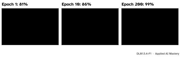
The 2-16-16-2 network on the two moons after 1, 10 and 200 epochs. Every bend in the vermillion curve was put there by gradients that the module library computed.
Each pass over the training set is an epoch. Before the first one, the random starting weights put every training point in the same class. After one epoch the boundary is a few straight pieces that still cut through both moons. Gradient steps then fold it, a little at a time, until it follows the gap between the moons.
Build it up
Step 1. The data. The course’s two-class set, \({\texttt{make\_moons}(200, \text{noise} = 0.2)}\) with random_state=0, split with stratification into 150 training and 50 validation points: 75 and 25 of each class.
Step 2. The network. Linear(2, 16), ReLU, Linear(16, 16), ReLU, Linear(16, 2), and the fused softmax cross-entropy. Its parameters, weights plus biases layer by layer, number
Step 3. The start. Weights are drawn from a normal distribution with standard deviation \({\sqrt{2/n_{\text{in}}}}\), where \(n_{\text{in}}\) is the number of inputs of the layer, and biases start at zero. Why this scale, and why the weights must not all be equal, is the subject of DL02.3; the pitfalls below show the second point.
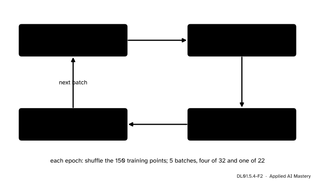
Step 4. One iteration.
DL01.5.4-F2
One iteration of the loop. The update is the only new line: everything else is the forward and backward of DL01.5.2.
Step 5. One epoch. Shuffle the 150 training indices, cut them into batches of 32, and run one iteration per batch. \({150} = {4 \times 32 + 22}\), so an epoch is five updates, the last on a short batch. After the epoch, measure the loss and the accuracy on the whole training set and on the validation set.
The formal statement
NoteMini-batch gradient descent (ML01.5.4)
Let \(\theta\) stand for all the weights and biases. For a batch \(B\) of example indices, with \({L_B(\theta)} = {\frac{1}{\abs{B}}\sum_{i \in B} \ell_i(\theta)}\), one update is
applied to every parameter at once, with the gradient computed by one forward and one backward pass at the current \(\theta\).
Backpropagation supplies \({\nabla_\theta L_B}\), already divided by \({\abs{B}}\) because the loss module returns \({(\mat{P} - \mat{Y})/\abs{B}}\). A short last batch therefore gives a gradient of the same size as a full one, not a smaller one.
How much should one step lower the loss? Write \(\vect{g}\) for the gradient, flattened into one vector. To first order (the linear approximation of M05.2),
The step lowers the loss by about \(\eta\) times the squared length of the gradient, as long as \(\eta\) is small enough for the linear approximation to hold. The worked example tests this.
DL01.5.4-F3
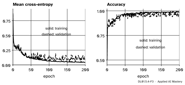
Training (solid) and validation (dashed) curves of the run. Both losses fall together at first. Later the training loss keeps falling while the validation loss levels off near 0.1 and wanders: the network is starting to fit the noise of its 150 points (ML01.8).
Worked example
One step of gradient descent on the running network of DL01.5.1, by hand, with \({\eta} = {0.02}\).
DL01.5.4-F4
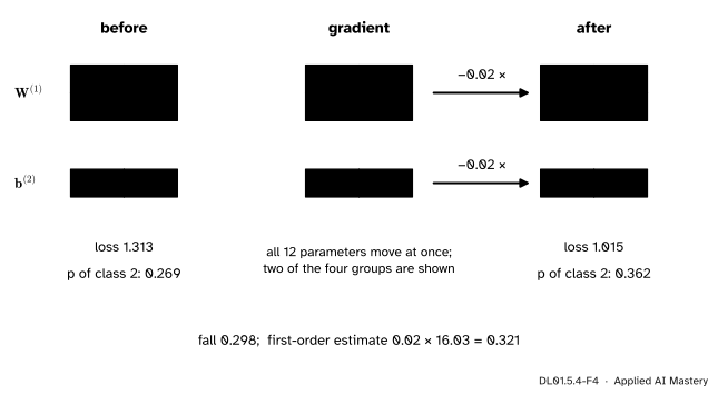
One update, before and after. All twelve parameters move at once; the weight with the largest gradient, \({w^{(1)}_{12}}\), moves most.
The update. Every parameter moves by \({-0.02}\) times its gradient. For two of them: \({w^{(1)}_{12}} \leftarrow {-0.5 - 0.02 \times 2.924} = {-0.558}\) and \({b^{(2)}_2} \leftarrow {0 - 0.02 \times (-0.731)} = {0.015}\). The rest follow the same rule.
The prediction. The squared length of the gradient is the sum of the squares of all twelve entries:
for \(\mat{W}^{(1)}\), \(\vect{b}^{(1)}\), \(\mat{W}^{(2)}\) and \(\vect{b}^{(2)}\) in turn. The first-order estimate of the fall is \({0.02 \times 16.03} \approx {0.321}\).
The check. Run the forward pass again with the new parameters: the probability of class 2 rises from 0.269 to 0.362 and the loss falls from 1.313 to 1.015, a fall of 0.298. The estimate was close; the small difference is the curvature that the linear approximation ignores. With \({\eta} = {0.1}\) the same step would be large enough to switch hidden unit 1 off, a reminder that the step size matters.
Code
The library of DL01.5.2, made general enough for any layer sizes, is in the folded cell.
The modules of DL01.5.2
import numpy as npclass Linear:def__init__(self, W, b):self.W, self.b = np.array(W, float), np.array(b, float)def forward(self, A):self.A = Areturn A @self.W.T +self.bdef backward(self, G):self.dW, self.db = G.T @self.A, G.sum(axis=0)return G @self.Wdef params(self):return [(self.W, "dW"), (self.b, "db")]class ReLU:def forward(self, Z):self.mask = Z >0return Z *self.maskdef backward(self, G):return G *self.maskdef params(self):return []class SoftmaxCrossEntropy:def forward(self, Z, labels): Z = Z - Z.max(axis=1, keepdims=True)self.P = np.exp(Z) / np.exp(Z).sum(axis=1, keepdims=True)self.Y = np.eye(Z.shape[1])[labels]return-np.mean(np.log(self.P[np.arange(len(labels)), labels]))def backward(self):return (self.P -self.Y) /len(self.P)class Sequential:def__init__(self, *layers):self.layers = layersdef forward(self, X):for layer inself.layers: X = layer.forward(X)return Xdef backward(self, G):for layer inreversed(self.layers): G = layer.backward(G)return G
The worked step first, on the running network.
net = Sequential(Linear([[1, -0.5], [-0.5, 1]], [0.5, -0.5]), ReLU(), Linear([[1, 1], [-1, 0.5]], [-0.5, 0]))x1, k1 = np.array([[1.0, 2.0]]), np.array([1])ce = SoftmaxCrossEntropy()before = ce.forward(net.forward(x1), k1)net.backward(ce.backward())grads = [getattr(m, name) for m in net.layers for _, name in m.params()]norm_sq =sum((g **2).sum() for g in grads)for m in net.layers:for P, name in m.params(): P -=0.02*getattr(m, name) # the update, in placeafter = ce.forward(net.forward(x1), k1)print(f"loss {before:.3f} -> {after:.3f}; fall {before - after:.3f}, first-order estimate {0.02* norm_sq:.3f}")
loss 1.313 -> 1.015; fall 0.298, first-order estimate 0.321
Now the loop. One generator draws the starting weights and then shuffles every epoch, so the run is the same every time; DL01.6.4 will repeat it step for step with its own engine.
import timefrom sklearn.datasets import make_moonsfrom sklearn.model_selection import train_test_splitX, y = make_moons(n_samples=200, noise=0.2, random_state=0)X_tr, X_va, y_tr, y_va = train_test_split(X, y, test_size=0.25, stratify=y, random_state=0)rng = np.random.default_rng(0)sizes = [2, 16, 16, 2]layers = []for n_in, n_out inzip(sizes[:-1], sizes[1:]): layers += [Linear(rng.normal(0, np.sqrt(2/ n_in), (n_out, n_in)), np.zeros(n_out)), ReLU()]net = Sequential(*layers[:-1]) # no ReLU after the last layern_params =sum(P.size for m in net.layers for P, _ in m.params())def evaluate(net, X, y): loss = SoftmaxCrossEntropy().forward(net.forward(X), y)return loss, np.mean(net.forward(X).argmax(axis=1) == y)lr, batch, epochs =0.2, 32, 200history = [evaluate(net, X_tr, y_tr) + evaluate(net, X_va, y_va)]start = time.perf_counter()for epoch inrange(epochs): order = rng.permutation(len(y_tr))for s inrange(0, len(y_tr), batch): idx = order[s:s + batch] loss_fn = SoftmaxCrossEntropy() loss_fn.forward(net.forward(X_tr[idx]), y_tr[idx]) # forward and loss net.backward(loss_fn.backward()) # backwardfor m in net.layers: # updatefor P, name in m.params(): P -= lr *getattr(m, name) history.append(evaluate(net, X_tr, y_tr) + evaluate(net, X_va, y_va))seconds = time.perf_counter() - starthistory = np.array(history) # columns: train loss, train acc, val loss, val accprint(f"{n_params} parameters, {epochs} epochs in {seconds:.2f} s")print("epoch 0: train loss %.3f acc %.2f | val loss %.3f acc %.2f"%tuple(history[0]))print("epoch 1: train loss %.3f acc %.2f | val loss %.3f acc %.2f"%tuple(history[1]))print("epoch 200: train loss %.3f acc %.2f | val loss %.3f acc %.2f"%tuple(history[-1]))print("lowest validation loss %.3f, at epoch %d"% (history[:, 2].min(), history[:, 2].argmin()))
354 parameters, 200 epochs in 0.07 s
epoch 0:   train loss 0.872 acc 0.50 | val loss 0.854 acc 0.50
epoch 1:   train loss 0.481 acc 0.81 | val loss 0.449 acc 0.82
epoch 200: train loss 0.042 acc 0.99 | val loss 0.128 acc 0.96
lowest validation loss 0.071, at epoch 172
The library version: scikit-learn’s MLPClassifier with the same hidden layers, solver, batch size and learning rate, on the same split.
hand-built: validation accuracy 0.96
MLPClassifier: validation accuracy 0.92 after 62 epochs
what it adds: alpha = 0.0001  momentum = 0.9  nesterovs_momentum = True  output: logistic
Both classifiers get most of the 50 validation points right; with 50 points, one point is 2 percent, so a difference of a few points is within the noise. The library is not plain SGD, though. Its defaults add an L2 penalty on the weights (alpha=0.0001), momentum with Nesterov’s correction (momentum=0.9), and a stopping rule that ends training when the loss has not improved by tol for n_iter_no_change=10 epochs, which is why it stopped early. For two classes it also uses one logistic output unit instead of two softmax units, an equivalent model (Exercise 2 of DL01.5.1). Momentum and penalties are DL02.1 and DL02.6.
Explore
Do one step of gradient descent yourself in the Backprop stepper of DL01.5.1. Run both passes, note the gradient of \({w^{(1)}_{12}}\), 2.924, and set that weight to \({-0.5 - 0.1 \times 2.924} \approx {-0.8}\). The loss falls, but hidden unit 1 is now off: a step of 0.1 on one weight already overshoots for that unit.
Pitfalls
DL01.5.4-F5
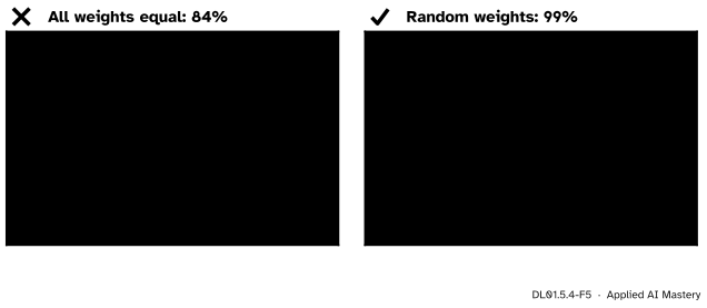
Wrong beside right. Start every weight at the same value and every hidden unit receives the same gradient, so the units stay identical forever and the network can only draw a straight boundary.
“The starting weights do not matter much; set them all to the same small number.”
If every weight of a layer is equal, every hidden unit computes the same value, receives the same gradient and takes the same step, so they stay equal for ever. Here all units of the first layer share one weight vector \(\vect{w}\) throughout, so the network sees only the single number \({\vect{w}\cdot\vect{x}}\). The units of the second layer stay identical too, so the difference of the two logits only ever rises, or only ever falls, as that number grows. The boundary is therefore a single straight line at right angles to \(\vect{w}\), however long the training runs: 84 percent on the training set, against 99 percent from random weights. Random starting weights break the symmetry; DL02.3 chooses their scale.
“A module can update its weights inside backward, as soon as it has the gradient.”
Linear’s backward returns \({\mat{G}\mat{W}}\), and that product must use the weights of the forward pass. Update \(\mat{W}\) first and the gradient handed to the layer below belongs to a different network. Finish the backward pass for every module, then update every parameter.
“The training loss is falling, so the network is getting better.”
It is getting better at the 150 training points. After about epoch 50 the training loss keeps falling while the validation loss levels off near 0.1 and wanders. The validation curve is the one that measures what the network has learned about moons in general, and it decides when to stop (ML01.8).
Check yourself
Recall
1. List the four steps of one training iteration.
Show answer
Forward the batch, compute the loss, backward to get every gradient, update every parameter by \({-\eta}\) times its gradient.
2. How many parameters does a 2-16-16-2 network have, and how?
Show answer
354: \({(32 + 16) + (256 + 16) + (32 + 2)}\), weights plus biases of the three layers.
3. How many updates make one epoch with 150 training points and batches of 32?
Show answer
Five: four batches of 32 and a last one of 22.
4. To first order, by how much does one gradient step lower the loss?
Show answer
By about \({\eta\norm{\vect{g}}^2}\), the learning rate times the squared length of the gradient.
5. Name two things that MLPClassifier(solver="sgd") adds by default that the hand-built loop does not have.
Show answer
Any two of: an L2 penalty (alpha=0.0001), momentum 0.9 with Nesterov’s correction, and a stopping rule that ends the run when the training loss has not improved by tol for 10 epochs.
Exercises
1.★ With 1,077 training images and batches of 64, how many updates are in one epoch, and how big is the last batch? How many updates do 30 epochs make?
Show solution
\({1077} = {16 \times 64 + 53}\), so an epoch has 17 updates, the last on 53 images. Thirty epochs make \({30 \times 17} = {510}\) updates.
2.★★ In the worked example, use the first-order estimate to find the step size that would, if the estimate held, lower the loss from 1.313 to 0.693. Then explain why the true loss after that step need not be 0.693.
Show solution
Solve \({0.693} = {1.313 - \eta \times 16.03}\): \({\eta} = {0.620/16.03} \approx {0.039}\). The estimate uses only the slope at the start. The loss curves, and a step this long also moves \({z^{(1)}_1}\) by about \({-0.039 \times 8.77} \approx {-0.34}\) (the change in \({\vect{w}^{(1)}_1 \cdot \vect{x} + b^{(1)}_1}\)), close to the ReLU’s kink at 0 where the linear picture of each unit changes. The true value has to be computed by a forward pass: it gives about 0.776, well above 0.693.
3.★★★ Show that if all the weights of the first hidden layer are equal and all its biases are equal, then every unit of that layer gets the same gradient for its weights, so after any number of gradient steps they are still equal. Assume the next layer’s weights start all equal too.
Show solution
With equal rows of \(\mat{W}^{(1)}\) and equal biases, every unit has the same pre-activation \({z_j} = {z}\) and the same activation. Suppose also that each row of \(\mat{W}^{(2)}\) has equal entries, which holds when all its weights are equal. Then the gradient arriving at each unit, \({(\mat{W}^{(2)\top}\vect{\delta}^{(2)})_j} = {\sum_i w^{(2)}_{ij}\delta^{(2)}_i}\), is the same for every \(j\), and so is the mask, so \({\delta^{(1)}_j}\) is the same for all \(j\). The gradient of row \(j\) of \(\mat{W}^{(1)}\) is \({\delta^{(1)}_j\vect{x}\T}\), the same row for every \(j\), and its bias gradient \({\delta^{(1)}_j}\) is the same too. Column \(j\) of \(\mat{W}^{(2)}\) gets \({\vect{\delta}^{(2)}a_j}\), the same for every \(j\), so each row of \(\mat{W}^{(2)}\) keeps equal entries. One update keeps both properties, so by induction they hold after every step. (Different rows of \(\mat{W}^{(2)}\) may drift apart; only the hidden units are tied.)
Summary card
Forward, loss, backward, update: repeat over shuffled batches.
DL01.5.4-F1
Gradients bend the boundary.
Update: \({\theta} \leftarrow {\theta - \eta\,\nabla_\theta L_B}\), after the whole backward pass.
One step lowers the loss by about \({\eta\norm{\vect{g}}^2}\).
2-16-16-2: 354 parameters; 150 points in batches of 32 is 5 updates per epoch.
Watch the validation curve, not only the training curve.
Sources and next steps
Sources. Each was opened and checked against this lesson on 15 November 2026.
S. J. D. Prince, Understanding Deep Learning (MIT Press, 2023), section 6.2.1: each iteration computes the gradient on a random batch, drawn without replacement, and updates the parameters by equation 6.10 (written with a sum over the batch; our mean only rescales the learning rate); one pass through the training set is an epoch. Section 7.4.1: the derivatives of every example in the batch are combined for the SGD update.
scikit-learn 1.9, MLPClassifier: alpha=0.0001 is the strength of the L2 term; momentum=0.9 and nesterovs_momentum=True are used when solver="sgd"; max_iter counts epochs for the stochastic solvers; training stops when the loss does not improve by at least tol for n_iter_no_change=10 consecutive epochs.
A. Zhang, Z. C. Lipton, M. Li and A. J. Smola, Dive into Deep Learning, section 5.3.4: backpropagation reuses the intermediate values stored by forward propagation, so they must be kept until backpropagation is complete.
Next. DL01.6 builds an autodiff engine that writes these backward passes for you and repeats this training run step for step; DL01.8 runs the same loop in PyTorch.