The PMF of one variable is hidden in the joint table: add each row for X and each column for Y. Why that is the law of total probability, why the margins cannot rebuild the table, and how summing out a hidden variable gives the mixture models of machine learning.
M06.9.2L1 Core25 minIn review (what this means)
The maths and code on this page are checked by automated tests on every change, but an independent reader has not signed it off yet. Spot a mistake or a confusing step? Tell us.
Find the marginal PMFs of a joint table as its row sums and column sums.
Derive the marginal formula from additivity and explain why it is the law of total probability, cell by cell.
Show with an example that the marginals do not determine the joint table.
Sum out a hidden variable to get the distribution of what is observed, as a mixture model does.
Compute marginals with NumPy axis sums and with pandas.crosstab and margins=True.
The question
The joint table of \(X\) and \(Y\) knows everything about the pair. So it must know the PMF of \(X\) on its own. Where in the table is it, and can we go the other way, rebuilding the table from the two PMFs? The answer explains a basic move of machine learning: when a model has a variable that is never observed, such as which cluster a point came from, it gets the distribution of the data by summing that variable out.
From the last lesson
1. On the course’s table, what is \({\Prob(X = Y)}\), and which cells give it?
2. Why is \({p(0, 2) = 0}\) in the course’s table?
Show answer
\({X = 0}\) needs flip 2 to be tails and \({Y = 2}\) needs it to be heads; no outcome does both.
Intuition
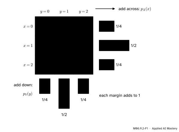
Every outcome with \({X = 1}\) sits somewhere in row \({x = 1}\), in one of its three cells. So the chance that \({X = 1}\) is the total of that row. Do this for every row and you have the PMF of \(X\); do it for every column and you have the PMF of \(Y\). Written in the margins of the table, these totals are called the marginal distributions.
M06.9.2-F1
Add across each row for the PMF of \(X\); add down each column for the PMF of \(Y\). For the course’s table both marginals are \(1/4\), \(1/2\), \(1/4\).
The table has nine numbers; each margin has three. Summing throws information away, and the lesson ends by asking what is lost.
Build it up
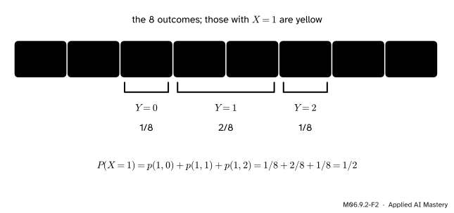
Step 1. Split one event by the other variable. The event \({X = 1}\) holds four outcomes: HTT, HTH, THT and THH. Sort them by their value of \(Y\) and they fall into three groups, one for each cell of row \({x = 1}\).
M06.9.2-F2
The event \({X = 1}\) is split by the value of \(Y\) into three disjoint pieces: the three cells of row 1.
Step 2. Add the pieces. The groups do not overlap, so additivity gives \({\Prob(X = 1)} = {1/8 + 2/8 + 1/8} = {1/2}\): the row total.
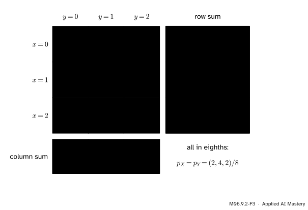
Step 3. Every row, then every column. The same split works for each value of \(X\), giving the row totals \(2/8\), \(4/8\), \(2/8\). Splitting each event \({Y = y}\) by the value of \(X\) gives the column totals, also \(2/8\), \(4/8\), \(2/8\).
Step 4. Try to go back. Suppose you were handed only the two margins, \({(1/4, 1/2, 1/4)}\) for each variable. Nine unknown cells must fit six totals, and the totals overlap: one of the six follows from the other five. Many tables fit, so the margins alone cannot say which table you had.
The formal statement
NoteMarginal PMFs
If \(X\) and \(Y\) have joint PMF \(p(x, y)\), the marginal PMFs of \(X\) and of \(Y\) are
The first sum runs over every value \(y\) of \(Y\): it adds row \(x\). The second adds column \(y\).
Why. Fix \(x\). Each outcome in the event \({X = x}\) has exactly one value of \(Y\), so the events \({X = x, Y = y}\), one for each \(y\), split \({X = x}\) into disjoint pieces with nothing left over. Additivity gives
The same argument with the roles swapped gives \(p_Y\).
It is the law of total probability. The events \({Y = y}\) form a partition of \(\Omega\), so the law of total probability (M06.3.3), with \({A = \{X = x\}}\) and \({B_y = \{Y = y\}}\), reads
\[
\begin{aligned}
&\Prob(X = x) \\
&= \sum_y \Prob(X = x \mid Y = y)\,\Prob(Y = y).
\end{aligned}
\]
By the multiplication rule each term is \({\Prob(X = x, Y = y)}\), a cell. So the row sum is the law of total probability with every leaf of the tree written straight into the table.
A marginal is a PMF. Its entries are sums of non-negative cells, so they are non-negative, and \({\sum_x p_X(x)} = {\sum_x \sum_y p(x, y)} = 1\), because that double sum adds the whole table.
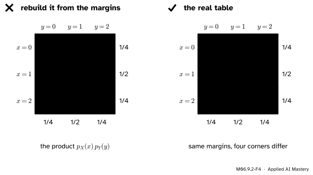
Marginals do not fix the joint. The course’s table and the product table, whose cells are \({p_X(x)\,p_Y(y)}\), have the same margins \({(1/4, 1/2, 1/4)}\) but differ in all four corners: the product table has \(1/16\) in each corner, the course’s table has \(2/16\), 0, 0 and \(2/16\). The middle cross of five cells agrees. The product table is the one an independent pair would have; lesson M06.9.3 makes that precise.
Go deeper: every table with the same margins, in one move
Take any table and pick two rows and two columns. Add a number \(d\) to two opposite corners of the rectangle they make, and subtract \(d\) from the other two corners. Each row and each column touched gains \(d\) once and loses it once, so every margin is unchanged. Starting from the product table and using the four corners with \({d = 1/16}\) gives
and likewise \({p(2, 2) = 2/16}\), \({p(2, 0) = 0}\): exactly the course’s table. Any \(d\) between \({-1/16}\) and \({1/16}\) keeps every cell non-negative and gives another valid table with the same margins, so there are infinitely many.
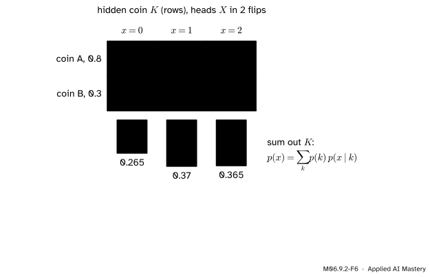
Summing out what you did not see. Often one of the two variables is never observed. Pick one of two coins at random, coin A with heads probability 0.8 or coin B with 0.3, each with chance \(1/2\), and flip the chosen coin twice. Let \(K\) be the coin and \(X\) the number of heads. The joint table has cells \({p(k, x)} = {p(k)\,p(x \mid k)}\). Someone who sees only the flips sees only the marginal of \(X\):
\[
p(x) = \sum_k p(k)\,p(x \mid k).
\]
M06.9.2-F6
A two-coin mixture. Each row is one coin’s PMF scaled by \(1/2\); the column sums are the distribution of the heads count when the coin is hidden.
That is a mixture: a weighted average of the coins’ PMFs. The Gaussian mixture models of ML03.4 work the same way, with clusters for coins and bell curves for PMFs. Their likelihood for each data point is a marginal, the hidden cluster summed out.
Worked example
Find both marginals of the course’s table and use one of them.
Rows. In eighths, the rows are \({(1, 1, 0)}\), \({(1, 2, 1)}\) and \({(0, 1, 1)}\):
Both margins of the course’s table, in eighths. The row sums and the column sums are the same, because swapping flips 1 and 3 swaps \(X\) and \(Y\).
Check. Each margin adds to \({2 + 4 + 2 = 8}\) eighths. And each matches what we know directly: \(X\) counts heads in two fair flips, so its PMF is \({\binom{2}{x}/4}\), which is \(1/4\), \(1/2\), \(1/4\) (M06.5.2).
Use it. A question about \(X\) alone needs only the margin: \({\Prob(X \leq 1)} = {p_X(0) + p_X(1)} = {3/4}\). Adding the six cells of rows 0 and 1 gives the same \(6/8\), with more work.
Code
From scratch, with the joint PMF as a dictionary from pairs to fractions: one loop adds each cell into the total for its \(x\) and the total for its \(y\).
import itertoolsfrom collections import Counter, defaultdictfrom fractions import Fractionimport numpy as npdef pair(word): h = [1if ch =="H"else0for ch in word]return h[0] + h[1], h[1] + h[2]outcomes = ["".join(w) for w in itertools.product("HT", repeat=3)]counts = Counter(pair(w) for w in outcomes)joint = {xy: Fraction(n, 8) for xy, n in counts.items()}p_X, p_Y = defaultdict(Fraction), defaultdict(Fraction)for (x, y), p in joint.items(): p_X[x] += p # the row total for x p_Y[y] += p # the column total for yprint("p_X:", [str(p_X[x]) for x inrange(3)])print("p_Y:", [str(p_Y[y]) for y inrange(3)])
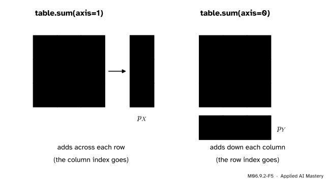
With the table as a NumPy array, the margins are one call each. The axis argument names the index that is summed away: axis=1 removes the column index, so each row collapses to its total.
M06.9.2-F5
The two axis sums. With rows for \(x\), axis=1 gives \(p_X\) and axis=0 gives \(p_Y\).
table = np.array([[1, 1, 0], [1, 2, 1], [0, 1, 1]]) /8# row x, column yproduct = np.outer(table.sum(axis=1), table.sum(axis=0)) # p_X(x) p_Y(y)print("p_X:", table.sum(axis=1), " p_Y:", table.sum(axis=0))print("product table x 16:\n", product *16)print("cells that differ:", [tuple(int(i) for i in c) for c in np.argwhere(~np.isclose(table, product))])coin = np.array([0.5, 0.5]) # p(k): coin A, coin Bgiven = np.array([[0.04, 0.32, 0.64], [0.49, 0.42, 0.09]]) # p(x | k), heads in two flipsmixture = (coin[:, None] * given).sum(axis=0) # sum out the hidden coinprint("mixture p(x):", mixture.round(3))
np.outer builds the product table from the two margins, and the comparison finds exactly the four corners. On data, pandas.crosstab with margins=True writes the margins into an extra row and column named All.
Y        0      1      2    All
X
0    0.128  0.125  0.000  0.253
1    0.123  0.252  0.122  0.497
2    0.000  0.124  0.126  0.250
All  0.250  0.501  0.248  1.000
The simulated margins sit within a couple of hundredths of \(1/4\), \(1/2\), \(1/4\).
Explore
The joint table explorer is in lesson M06.9.3. Its margins are drawn as bars along the edges of the table. Switch on the independent table and watch the bars stay exactly where they are while the four corners change.
Pitfalls
M06.9.2-F4
Wrong beside right. The product of the margins is one table with these margins; the real table is another. They differ in the four ringed corners.
“From the two marginals I can rebuild the joint table.”
Only if you also know that the variables are independent. The margins of the course’s table are the same as those of the product table, yet \({p(0, 2) = 0}\) against \(1/16\). In a data set, two columns with the same histograms can be linked in very different ways; summaries of single columns cannot reveal it.
“table.sum(axis=0) gives the marginal of the row variable.”
It gives the opposite. axis=0 sums over the row index, down each column, which leaves the column variable. With rows for \(x\), table.sum(axis=1) is \(p_X\). The course’s two margins are equal, so a mix-up would go unnoticed here; test on a table whose margins differ.
“Marginal means minor.”
Here it means “written in the margin”. A marginal distribution is a full PMF in its own right, often the one we care about most, as with the observed data in a mixture model.
Check yourself
Recall
1. How do you get \(p_X\) from a joint table whose rows are the values of \(X\)?
Show answer
Add each row: \({p_X(x) = \sum_y p(x, y)}\).
2. Which law of probability is the row sum a case of?
Show answer
The law of total probability, with the partition \({Y = y}\): each term \({\Prob(X = x \mid Y = y)\,\Prob(Y = y)}\) is one cell.
3. Give two different tables with margins \(1/4\), \(1/2\), \(1/4\) on both sides.
Show answer
The course’s table and the product table, whose cells are \({p_X(x)\,p_Y(y)}\) in sixteenths \({(1, 2, 1)}\), \({(2, 4, 2)}\), \({(1, 2, 1)}\).
4. With a NumPy array table whose rows are \(x\), which call gives \(p_Y\)?
Show answer
table.sum(axis=0), which adds down each column.
5. What does “summing out” a hidden variable \(K\) give?
Show answer
The marginal of what is observed, \({p(x) = \sum_k p(k)\,p(x \mid k)}\): a mixture.
Exercises
1.★ A joint table has rows \({x = 0, 1}\) and columns \({y = 0, 1, 2}\), with row 0 reading \({0.10, 0.20, 0.10}\) and row 1 reading \({0.30, 0.10, 0.20}\). Find both marginals and \({\Prob(Y \geq 1)}\).
2.★★ Let \(X\) be heads in two fair flips and set \({Y = X}\). Write the joint table, find its margins, and compare \({\Prob(X = Y)}\) with the course’s table.
Show solution
\({Y = X}\) always, so all the probability sits on the diagonal: \({p(0, 0) = 1/4}\), \({p(1, 1) = 1/2}\), \({p(2, 2) = 1/4}\), and every other cell is 0. The margins are \({(1/4, 1/2, 1/4)}\) for both, the same as the course’s table and the product table. But \({\Prob(X = Y) = 1}\) here, against \(1/2\) for the course’s table and \(3/8\) for the product table. Three tables, one pair of margins, three answers.
3.★★★ Two variables each take the values 0 and 1 with probability \(1/2\). Show that every joint table with these margins has the form with \({p(0, 0) = p(1, 1) = a}\) and \({p(0, 1) = p(1, 0) = 1/2 - a}\) for some \(a\) between 0 and \(1/2\), and find \({\Prob(X = Y)}\) in terms of \(a\).
Show solution
Let \({p(0, 0) = a}\). Row 0 must add to \(1/2\), so \({p(0, 1) = 1/2 - a}\). Column 0 must add to \(1/2\), so \({p(1, 0) = 1/2 - a}\). Row 1 must add to \(1/2\), so \({p(1, 1)} = {1/2 - (1/2 - a)} = a\), and then column 1 is \({(1/2 - a) + a} = {1/2}\), as it must be. Every cell is non-negative exactly when \({0 \leq a \leq 1/2}\). Then \({\Prob(X = Y)} = {p(0, 0) + p(1, 1)} = {2a}\), which can be anything from 0 to 1. The margins say nothing about it; the case \({a = 1/4}\) is the product table.
Summary card
Add across for \(p_X\), add down for \(p_Y\); the margins cannot rebuild the table.
MIT OpenCourseWare 18.05, Reading 7a, Joint Distributions, Independence, Spring 2022. Sections 3.6 and 3.7: row sums go in the right-hand margin and column sums in the bottom margin, and “the term marginal refers to the fact that the values are written in the margins of the table”.
NumPy reference, numpy.sum: axis names the axis along which the sum is performed; its example sums [[0, 1], [0, 5]] to [0, 6] with axis=0 and to [1, 5] with axis=1.
pandas reference, pandas.crosstab: margins=True adds row and column subtotals in a row and column named All, and with normalize the margin values are normalised too.