Geometric and exponential: waiting for the first success
How many trials until the first success, and how long until the next event? Derive the geometric PMF and its mean 1/p, pack ever more trials into each minute to reach the exponential wait e^(-lambda t), and prove that both forget how long you have waited.
M06.8.2L1 Core25 minIn review (what this means)
The maths and code on this page are checked by automated tests on every change, but an independent reader has not signed it off yet. Spot a mistake or a confusing step? Tell us.
Derive the geometric PMF (1 - p)^(k - 1) p and its tail (1 - p)^k from the story of trials up to the first success.
Derive the mean 1/p by differentiating the geometric series.
Obtain the exponential tail e^(-lambda t) as the limit of geometric waits with ever shorter trials, and its mean 1/lambda by integration by parts.
Prove that the geometric and exponential distributions are memoryless, and explain what that does and does not imply.
Compute waiting-time probabilities by hand, by simulation and with scipy.stats.geom and expon, giving expon its scale 1/lambda.
The question
Random search tries hyperparameter settings one after another, and each try lands in the best 5% of settings with chance 0.05. How many tries should you expect to need, and how likely is it that 60 tries are not enough? A server receives requests at an average rate of 0.5 per minute. How long until the next one, and does the answer change if none has come for 4 minutes?
From the last lesson
1. What is the PMF of \({\mathrm{Bin}(n, p)}\), and where does each factor come from?
Show answer
\({\binom{n}{k} p^k (1 - p)^{n-k}}\): the number of sequences with \(k\) successes, times the chance of each such sequence.
2. What are the mean and variance of \({\mathrm{Bin}(n, p)}\)?
Show answer
\({np}\) and \({np(1 - p)}\).
Intuition
The binomial fixed the number of trials and counted successes. Now keep going until the first success and count the trials it took. That number is a waiting time.
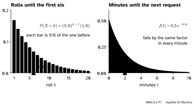
M06.8.2-F1
Two waits for a first success. Left: rolls of a die until the first six, a geometric distribution. Right: minutes until the next request at 0.5 per minute, an exponential density. Each shrinks by a fixed factor per step: the same shape, in whole trials and in continuous time.
Both pictures fall away steadily, and for the same reason. To wait longer than \(k\) steps, every one of the first \(k\) steps must fail, and each failure multiplies the chance by the same factor.
Build it up
Step 1. The tail. Let \(X\) be the number of trials up to and including the first success, with success chance \(p\) on each independent trial. “\({X > k}\)” says that the first \(k\) trials all failed, so by independence, for \({k = 0, 1, 2, \ldots}\),
\[
\Prob(X > k) = (1 - p)^k .
\]
Step 2. The PMF. “\({X = k}\)” says that the first \({k - 1}\) trials failed and trial \(k\) succeeded. For \({k = 1, 2, \ldots}\),
\[
\Prob(X = k) = (1 - p)^{k-1}\, p .
\]
For a die and a six, \({p = 1/6}\), so \({\Prob(X = 3)} = {(5/6)^2 (1/6)} = {25/216} \approx 0.116\).
Step 3. The bars add to 1. With \({q = 1 - p}\), the bars form a geometric series with ratio \(q\), and \({0 \le q < 1}\) when \({p > 0}\) (M04.8.1):
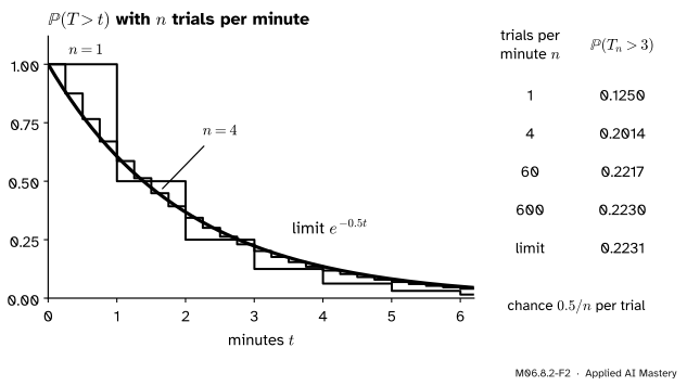
Step 4. Shorter and shorter trials. A server’s requests do not come in trials, but we can pretend they do. Cut each minute into \(n\) short slots, and let each slot hold a request with chance \({0.5/n}\), so that the average stays 0.5 requests per minute. The wait in minutes is \({T_n = X_n / n}\), where \(X_n\) is a geometric number of slots. Waiting more than 3 minutes means that the first \({3n}\) slots are empty:
Packing more trials into each minute. With one trial a minute the tail is a coarse staircase; with 4 it is finer; as \(n\) grows it settles onto the smooth curve \({e^{-0.5t}}\).
With one slot per second (\({n = 60}\)) the answer is 0.2217; with \({n = 600}\) it is 0.2230. The numbers settle on \({e^{-1.5} = 0.2231}\), and the formal statement shows why.
The formal statement
NoteDefinition: geometric and exponential distributions
\({X \sim \mathrm{Geom}(p)}\) counts the independent trials, each a success with chance \(p\), up to and including the first success. For \({k = 1, 2, \ldots}\),
\[
p_X(k) = (1 - p)^{k-1} p .
\]
Its tail is \({\Prob(X > k) = (1 - p)^k}\) and its mean is \({1/p}\).
\({T \sim \mathrm{Exp}(\lambda)}\), with a rate \({\lambda > 0}\) of events per unit of time, has
Its tail is \({\Prob(T > t) = e^{-\lambda t}}\) and its mean is \({1/\lambda}\).
In scipy.stats these are geom(p), which counts trials from 1 as here, and expon(scale=1/λ): SciPy describes the exponential by its mean, called the scale, not by its rate.
The mean of the geometric. For \({\abs{q} < 1}\) the geometric series gives \({\sum_{k=0}^{\infty} q^k = 1/(1 - q)}\). A power series may be differentiated term by term inside the interval where it converges (a theorem of analysis that we use without proof here; the box below reaches the same mean without it), so differentiating both sides in \(q\) gives
With a one-in-six chance you wait 6 rolls on average; with 0.05 you wait 20 tries.
Go deeper: the same mean without differentiating
For a variable with values \({1, 2, \ldots}\), let \(I_k\) be the indicator of the event \({X \ge k}\). Then \({X = I_1 + I_2 + \cdots}\): the indicators for \({k = 1, \ldots, X}\) are 1 and the rest are 0. The terms are never negative, so the expectation of the sum is the sum of the expectations, and
Proof. For \({x = 0}\) both sides are 1. Otherwise, once \({n > \abs{x}}\) the bracket is positive, so we may take logarithms. Put \({h = x/n}\), which tends to 0:
\[
\begin{aligned}
n \ln\Big(1 + \frac{x}{n}\Big) &= x \cdot \frac{\ln(1 + h) - \ln 1}{h} \\
&\to x \cdot \frac{d}{dy}\ln y \,\Big|_{y=1} \\
&= x \cdot 1 = x .
\end{aligned}
\]
The quotient is a difference quotient of \({\ln}\) at 1, and the derivative of \({\ln y}\) is \({1/y}\) (M04.3.4). Since \({e^y}\) is continuous, \({(1 + x/n)^n = e^{n \ln(1 + x/n)} \to e^x}\).
The tail. With \(n\) slots per unit of time, each holding an event with chance \({\lambda/n}\), waiting longer than \(t\) means that the first \({nt}\) slots are empty. Take \(t\) with \({nt}\) a whole number; the general case changes the exponent by less than 1, a factor that tends to 1. Then
by the lemma with \({x = -\lambda}\). So the limiting wait has CDF \({F(t) = 1 - e^{-\lambda t}}\) for \({t \ge 0}\), and its density is the derivative (M06.6.3): \({f(t) = \lambda e^{-\lambda t}}\).
The mean of the exponential. Integrate by parts (M04.7.2) with \({u = t}\) and \({dv = \lambda e^{-\lambda t}\,dt}\), so that \({v = -e^{-\lambda t}}\):
The bracket is 0 at both ends because \({t e^{-\lambda t} \to 0}\) as \({t \to \infty}\); the last integral is \({[-e^{-\lambda t}/\lambda]_0^\infty = 1/\lambda}\). At 0.5 requests per minute the mean wait is 2 minutes.
Both forget the past. Suppose the first \(m\) trials have failed. The chance of \(k\) more failures is, since \({\{X > m + k\}}\) lies inside \({\{X > m\}}\),
\[
\begin{aligned}
&\Prob(X > m + k \mid X > m) \\
&\quad= \frac{\Prob(X > m + k)}{\Prob(X > m)} \\
&\quad= \frac{q^{m+k}}{q^m} = q^k = \Prob(X > k) .
\end{aligned}
\]
The same steps with \({e^{-\lambda t}}\) in place of \({q^k}\) give
\[
\begin{aligned}
&\Prob(T > s + u \mid T > s) \\
&\quad= e^{-\lambda u} = \Prob(T > u) .
\end{aligned}
\]
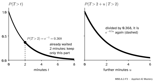
This is the memoryless property: having waited tells you nothing about how much longer you will wait.
M06.8.2-F3
Memorylessness as a picture. Keep the part of the tail after 2 minutes and rescale it to start at 1: it is the whole tail again.
Worked example
Requests arrive at \({\lambda = 0.5}\) per minute, so the wait is \({T \sim \mathrm{Exp}(0.5)}\). Find the chance of waiting more than 3 minutes, of a request within 1 minute, and the median wait. Then check the first answer with one trial per second.
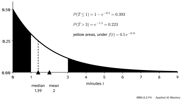
More than 3 minutes.\({\Prob(T > 3) = e^{-0.5 \times 3} = e^{-1.5} = 0.2231}\).
The median. Solve \({\Prob(T > m) = \tfrac12}\): \({e^{-0.5m} = \tfrac12}\), so \({m = \ln 2 / 0.5 = 1.386}\) minutes. Half of all waits are shorter than 1.39 minutes, though the mean is 2: a few long waits pull the mean up.
M06.8.2-F4
The worked example as areas under the density. The median, where the area splits in half, sits left of the mean.
One trial per second. With \({n = 60}\) slots per minute, each with chance \({0.5/60 = 1/120}\), three minutes are 180 slots, and \({\Prob(T_{60} > 3)} = {(1 - 1/120)^{180}} = 0.2217\). The geometric answer is within 0.0014 of the exponential one.
Memoryless. If no request has come for 2 minutes, the chance of waiting 3 more is still 0.2231. And for random search, \({X \sim \mathrm{Geom}(0.05)}\): the mean is \({1/0.05 = 20}\) tries, and \({\Prob(X > 60) = 0.95^{60} = 0.0461}\).
Code
From scratch: the geometric PMF and its partial sums, which should settle on 1 and on the mean \({1/p}\).
P(X = 3) = 25/216   P(X > 6) = 15625/46656 = 0.3349
first 300 bars add to 1.0  mean so far: 6.0
random search: P(X > 60) = 0.0461   mean = 20.0
exponential: 0.2231 0.3935 1.386
one slot per second: 0.2217
A simulation that runs the trials one by one, then NumPy’s samplers. rng.geometric counts trials from 1, and rng.exponential also takes the scale \({1/\lambda}\).
import numpy as nprng = np.random.default_rng(seed=1)def trials_until_success(p): k =1while rng.random() >= p: # a failure: try again k +=1return kby_hand = np.array([trials_until_success(1/6) for _ inrange(20_000)])fast = rng.geometric(p=0.05, size=200_000)waits = rng.exponential(scale=2.0, size=200_000) # rate 0.5, so scale 2print("die:", by_hand.mean().round(2), " search:", fast.mean().round(2), (fast >60).mean().round(4))print("waits:", waits.mean().round(3), (waits >3).mean().round(4))print("memoryless:", ((waits >5).sum() / (waits >2).sum()).round(4))
Among the simulated waits longer than 2 minutes, the share that also last past 5 is about 0.223, the same as the share of all waits that last past 3. Last, SciPy:
from scipy import statsG = stats.geom(0.05) # trials up to and including the first successT = stats.expon(scale=1/0.5) # scale = 1/lambda = 2 minutesprint(G.mean(), round(G.sf(60), 4), round(T.sf(3), 4), round(T.cdf(1), 4), round(T.median(), 3), T.mean())
20.0 0.0461 0.2231 0.3935 1.386 2.0
sf is the survival function, \({\Prob(X > x)}\): the tail of this lesson.
Explore
The module’s interactive, the distribution map, lives in lesson M06.8.4. Choose the arrow from geometric to exponential and step the number of trials per minute up from 1: the staircase closes in on the curve.
Pitfalls
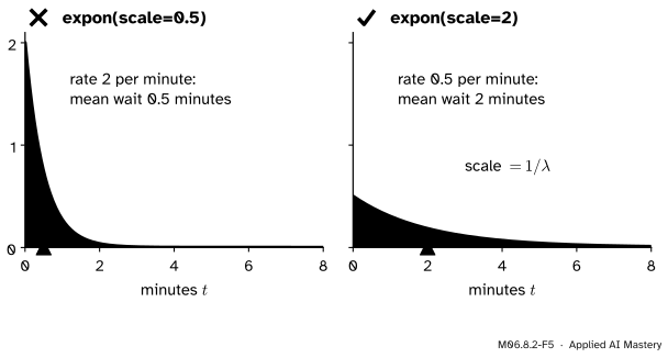
M06.8.2-F5
Wrong beside right. Passing the rate 0.5 as SciPy’s scale builds a wait four times too short on average. The scale is the mean, \({1/\lambda}\).
“stats.expon(scale=0.5) is the exponential with rate 0.5.”
SciPy and NumPy describe the exponential by its scale, the mean \({1/\lambda}\). Rate 0.5 per minute is scale=2. The mistake is silent: every number comes out, and all of them are wrong.
“No request for 4 minutes, so one is due any moment.”
Under the exponential story the chance of a request in the next minute is \({1 - e^{-0.5} = 0.39}\) whatever has happened before. If a process really does become more likely to fire the longer it waits, such as a part wearing out, the exponential is the wrong family.
“The geometric mean is \({(1 - p)/p}\).”
That is the mean number of failures before the first success, a different count that takes the value 0 when the first trial succeeds. This course, SciPy’s geom and NumPy’s geometric all count trials from 1, with mean \({1/p}\). Check which count a book or library means before using its formulas.
Check yourself
Recall
1. For \({X \sim \mathrm{Geom}(p)}\), what are \({\Prob(X > k)}\) and \({\Prob(X = k)}\)?
Show answer
\({(1 - p)^k}\), since the first \(k\) trials all fail; and \({(1 - p)^{k-1} p}\), since \({k - 1}\) failures are followed by a success.
2. What is the mean of \({\mathrm{Geom}(p)}\), and how is it derived here?
Show answer
\({1/p}\), by differentiating \({\sum q^k = 1/(1 - q)}\) to get \({\sum k q^{k-1} = 1/(1 - q)^2}\) and setting \({q = 1 - p}\).
3. Which limit turns geometric waits into the exponential tail?
Show answer
\({(1 + x/n)^n \to e^x}\), used with \({x = -\lambda}\) on \({(1 - \lambda/n)^{nt}}\).
4. State the memoryless property of the exponential.
Show answer
\({\Prob(T > s + u \mid T > s)} = {\Prob(T > u)}\) for all \({s, u \ge 0}\).
5. How do you build \({\mathrm{Exp}(\lambda)}\) in scipy.stats?
Show answer
stats.expon(scale=1/lam): the scale is the mean \({1/\lambda}\), not the rate.
Exercises
1.★ A fair die is rolled until the first six. Find the chance that this takes exactly 3 rolls, the chance that it takes more than 6 rolls, and the mean number of rolls.
Show solution
\(X \sim \mathrm{Geom}(1/6)\), so \({\Prob(X = 3)} = {(5/6)^2 (1/6)} = {25/216} = 0.116\), and \({\Prob(X > 6)} = {(5/6)^6} = 0.335\): in a third of games, six rolls are not enough, though the mean is \({1/p = 6}\).
2.★★ Show that \({\mathrm{Var}(X) = (1 - p)/p^2}\) for \({X \sim \mathrm{Geom}(p)}\).
Show solution
Differentiate \({\sum_{k \ge 1} k q^{k-1} = (1 - q)^{-2}}\) once more: \({\sum_{k \ge 2} k(k - 1) q^{k-2} = 2(1 - q)^{-3}}\). Then
The bracket is 0 at both ends, and the last integral is \({\E[T] = 1/\lambda}\). So \({\mathrm{Var}(T) = 2/\lambda^2 - (1/\lambda)^2 = 1/\lambda^2}\), and the standard deviation equals the mean: 2 minutes at 0.5 requests per minute.
Summary card
Waiting for a first success: geometric in trials, exponential in continuous time, and both forget the past.
The bridge.\({(1 - \lambda/n)^{nt} \to e^{-\lambda t}}\).
SciPy.stats.geom(p), stats.expon(scale=1/lam).
Sources and next steps
Sources. Each was opened and checked against this lesson on 14 November 2026.
Hossein Pishro-Nik, Introduction to Probability, Statistics, and Random Processes, Section 3.1.5: the geometric PMF \({p(1 - p)^{k-1}}\) for tosses up to and including the first heads, with a note that some books count only the failures. Section 3.2.2 finds the mean \({1/p}\) by differentiating the geometric sum. Section 4.2.2 gives the exponential density, CDF, mean \({1/\lambda}\), variance \({1/\lambda^2}\), the memoryless property, and the exponential as the limit of geometric waits with tosses every \(\Delta\) seconds.
SciPy developers, scipy.stats.geom, with PMF \({(1 - p)^{k-1} p}\) for \({k \ge 1}\), and scipy.stats.expon, whose rate form \({\lambda e^{-\lambda x}}\) “corresponds to using scale = 1 / lambda” (SciPy 1.18).
NumPy developers, Generator.geometric, supported on \({k = 1, 2, \ldots}\), and Generator.exponential, whose scale is the inverse of the rate (NumPy 2.5 reference).
Next.M06.8.3 Poisson: counting rare events uses the same slots and the same limit, but counts the events in a window instead of waiting for the first.